Differential Expression with edgeR
Differential Expression mini lecture
If you would like a brief refresher on differential expression analysis, please refer to the mini lecture.
edgeR DE Analysis
In this tutorial you will:
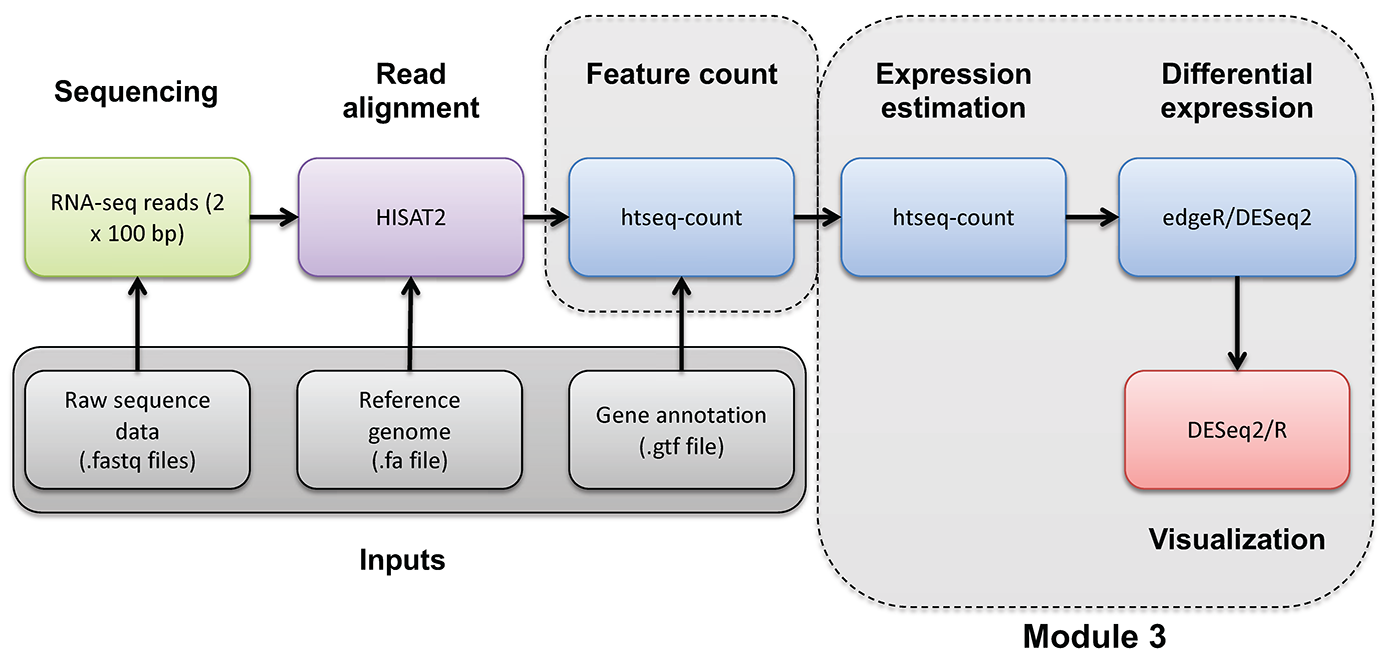
- Make use of the raw counts you generated previously using htseq-count
- edgeR is a bioconductor package designed specifically for differential expression of count-based RNA-seq data
- This is an alternative to using stringtie/ballgown to find differentially expressed genes
First, create a directory for results:
cd $RNA_HOME/
mkdir -p de/htseq_counts/edgeR
cd de/htseq_counts/edgeR
Launch R:
R
R code has been provided below. If you wish to have a script with all of the code, it can be found here. Run the R commands below.
# set working directory where output will go
working_dir = "~/workspace/rnaseq/de/htseq_counts/edgeR"
setwd(working_dir)

# read in gene mapping
mapping = read.table("~/workspace/rnaseq/de/htseq_counts/ENSG_ID2Name.txt", header = FALSE, stringsAsFactors = FALSE, row.names = 1)

# read in count matrix
rawdata = read.table("~/workspace/rnaseq/expression/htseq_counts/gene_read_counts_table_all_final.tsv", header = TRUE, stringsAsFactors = FALSE, row.names = 1)

# Check dimensions
dim(rawdata)

# Require at least 1/6 of samples to have expressed count >= 10
sample_cutoff = (1/6)
count_cutoff = 10

#Define a function to calculate the fraction of values expressed above the count cutoff
getFE = function(data,count_cutoff){
 FE = (sum(data >= count_cutoff) / length(data))
 return(FE)
}

#Apply the function to all genes, and filter out genes not meeting the sample cutoff
fraction_expressed = apply(rawdata, 1, getFE, count_cutoff)
keep = which(fraction_expressed >= sample_cutoff)
rawdata = rawdata[keep, ]

# Check dimensions again to see effect of filtering
dim(rawdata)

#################
# Running edgeR #
#################

# load edgeR
library("edgeR")

# make class labels
class = c(rep("UHR", 3), rep("HBR", 3))

# Get common gene names
Gene = rownames(rawdata)
Symbol = mapping[Gene, 1]
gene_annotations = cbind(Gene, Symbol)

# Make DGEList object
y = DGEList(counts = rawdata, genes = gene_annotations, group = class)
nrow(y)

# TMM Normalization
y = calcNormFactors(y)

# Estimate dispersion
y = estimateCommonDisp(y, verbose = TRUE)
y = estimateTagwiseDisp(y)

# Differential expression test
et = exactTest(y)

# Extract raw counts to add back onto DE results
counts = getCounts(y)

# Print top genes
topTags(et)

# Print number of up/down significant genes at FDR = 0.05  significance level
summary(de <- decideTests(et, adjust.method = "BH", p = 0.05))

#Get output with BH-adjusted FDR values - all genes, any p-value, unsorted
out = topTags(et, n = "Inf", adjust.method = "BH", sort.by = "none", p.value = 1)$table

#Add raw counts back onto results for convenience (make sure sort and total number of elements allows proper join)
out2 = cbind(out, counts)

#Limit to significantly DE genes
out3 = out2[as.logical(de), ]

# Order by p-value
o = order(et$table$PValue[as.logical(de)], decreasing=FALSE)
out4 = out3[o, ]

# Save table
write.table(out4, file = "DE_sig_genes_edgeR.tsv", quote = FALSE, row.names = FALSE, sep = "\t")

#To exit R type the following
quit(save = "no")