Differential Expression with DESeq2
Differential Expression mini lecture
If you would like a brief refresher on differential expression analysis, please refer to the mini lecture.
DESeq2 DE Analysis
In this tutorial you will:
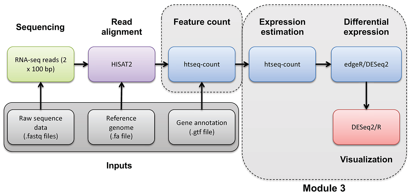
- Make use of the raw counts you generated previously using htseq-count
- DESeq2 is a bioconductor package designed specifically for differential expression of count-based RNA-seq data
- This is an alternative to using stringtie/ballgown to find differentially expressed genes
Setup
Here we start from within an R session, relevant packages should already be installed so we will load the libraries, set working directories and read in the raw read counts data. Two pieces of information are required to perform analysis with DESeq2. A matrix of raw counts, such as was generated previously while running HTseq previously in this course. This is important as DESeq2 normalizes the data, correcting for differences in library size using using this type of data. DESeq2 also requires the experimental design which can be supplied as a data.frame, detailing the samples and conditions.
# define working dir paths
datadir = "/home/ubuntu/workspace/rnaseq/expression/htseq_counts/"
outdir = "/home/ubuntu/workspace/rnaseq/de/htseq_counts/deseq2/"

# load R libraries we will use in this section - suppress some harmless warnings from the data.table package
library(DESeq2)
suppressPackageStartupMessages(library(data.table))
library(ggplot2)

# set working directory to data dir
setwd(datadir)

# create our output directory, if it doesn't already exist
if (!dir.exists(outdir)) dir.create(outdir)

# read in the RNAseq read counts for each gene (produced by htseq-count)
htseqCounts = fread("gene_read_counts_table_all_final.tsv")
Once we start from R, the relevant packages should already be installed. We will load the libraries, set working directories, and read in the raw read counts data. Two pieces of information are required to perform analysis with DESeq2. A matrix of raw counts, such as was generated previously while running HTseq previously in this course. This is important as DESeq2 normalizes the data, correcting for differences in library size using using this type of data. DESeq2 also requires the experimental design which can be supplied as a data.frame, detailing the samples and conditions.
Format htseq counts data to work with DESeq2
DESeq2 has a number of options for data import and has a function to read HTseq output files directly. Here the most universal option is used, reading in raw counts from a matrix in simple TSV format (one row per gene, one column per sample). The HTseq count data that was read in above is stored as an object of class “data.table”, this can be verified with the class() function. Before use in this exercise it is required to convert this object to an appropriate matrix format with gene names as rows and samples as columns.
It should be noted that while the replicate samples are technical replicates (i.e. the same library was sequenced), herein they are treated as biological replicates for illustrative purposes. DESeq2 does have a function to collapse technical replicates though.
# view the class of the data
class(htseqCounts)

# convert the data.table to matrix format
htseqCounts = as.matrix(htseqCounts)
class(htseqCounts)

# set the gene ID values to be the row names for the matrix
rownames(htseqCounts) = htseqCounts[, "GeneID"]

# now that the gene IDs are the row names, remove the redundant column that contains them
htseqCounts = htseqCounts[, colnames(htseqCounts) != "GeneID"]

# convert the count values from strings (with spaces) to integers, because originally the gene column contained characters, the entire matrix was set to character
class(htseqCounts) = "integer"

# view the first few lines of the gene count matrix
head(htseqCounts)
Filter raw counts
Before running DESeq2 (or any differential expression analysis) it is useful and common practice to pre-filter the data. There are computational benefits to doing this as the memory size of the objects within R will decrease and DESeq2 will have less data to work through and will be faster. More importantly, by removing “low quality” data, it is also reduces the number of statistical tests that will be performed, which in turn reduces the impact of multiple test correction and can lead to more significant genes.
The amount of pre-filtering is up to the analyst. However, it must be done in an unbiased way (i.e. you can NOT remove genes that don’t have a difference between conditions of interest, or that show an unexpected pattern).
DESeq2 recommends removing any gene with less than 10 reads across all samples. Below, we filter a gene if at least 1 sample does not have at least 10 reads. Either way, mostly what is being removed here are genes with very little evidence for expression in any sample (in many cases genes with 0 counts in all samples).
# run a filtering step
# i.e. require that for every gene: at least 1 of 6 samples must have counts greater than 10
# get the index of rows that meet this criterion and use that to create a subset of the matrix
# note the dimensions of the matrix before and after filtering with dim()

# breaking apart the command below to understand it's outcome
tail(htseqCounts) # look at the raw counts
tail(htseqCounts >= 10) # determine which cells have counts greater than 10
tail(rowSums(htseqCounts >= 10)) # for each gene row, count how many samples have a count greater than 10
tail(rowSums(htseqCounts >= 10) >= 1) # filter to those genes where at least one sample has a count greater than 10
tail(which(rowSums(htseqCounts >= 10) >= 1)) #obtain the index for rows that meet the above filter criteria

dim(htseqCounts)
htseqCounts = htseqCounts[which(rowSums(htseqCounts >= 10) >= 1), ]
dim(htseqCounts)
Specifying the experimental design
As mentioned above DESeq2 also needs to know the experimental design. In our experimental design this means which samples belong to which condition. The experimental design for the example dataset is quite simple as there are 6 samples with two conditions to compare (UHR vs HBR). We can create the experimental design right within R. There is one important thing to note, DESeq2 does not check sample names, it expects that the column names in the counts matrix we created correspond exactly to the row names we specify in the experimental design.
# construct a mapping of the meta data for our experiment (comparing UHR cell lines to HBR brain tissues)
# this is defining the biological condition/label for each experimental replicate
# create a simple one column dataframe to start
metaData <- data.frame("Condition" = c("UHR", "UHR", "UHR", "HBR", "HBR", "HBR"))

# convert the "Condition" column to a factor data type
# the arbitrary order of these factors will determine the direction of log2 fold-changes for the genes (i.e. up or down regulated)
# the condition that is listed second here will correspond to a +ve log2 fold change
# genes with counts higher in UHR will have a fold change > 1, or +ve log2 fold change
# genes with counts higher in HBR will have a fold change < 1 (fractions), or -ve log2 fold change

metaData$Condition = factor(metaData$Condition, levels = c("HBR", "UHR"))

# set the row names of the metaData dataframe to be the names of our sample replicates from the read counts matrix
rownames(metaData) = colnames(htseqCounts)

# view the metadata dataframe
head(metaData)

# check that names of htseq count columns match the names of the meta data rows
# use the "all" function which tests whether an entire logical vector is TRUE
all(rownames(metaData) == colnames(htseqCounts))
Construct the DESeq2 object piecing all the data together
With all the data properly formatted it is now possible to combine all the information required and run the differental expression analysis in one object. This object will hold the input data, and intermediary calculations. It is also where the condition to test is specified.
# make deseq2 data sets
# here we are setting up our experiment by supplying: (1) the gene counts matrix, (2) the sample/replicate for each column, and (3) the biological conditions we wish to compare.
# this is a simple example that works for many experiments but these can also get more complex
# for example, including designs with multiple variables such as "~ group + condition",
# and designs with interactions such as "~ genotype + treatment + genotype:treatment".

dds = DESeqDataSetFromMatrix(countData = htseqCounts, colData = metaData, design = ~Condition)

# the design formula above is often a point of confusion, it is useful to put in words what is happening, when we specify "design = ~Condition" we are saying
# regress gene expression on condition, or put another way, model gene expression on condition
# gene expression is the response variable and condition is the explanatory variable
# you can put words to formulas using this [cheat sheet](https://www.econometrics.blog/post/the-r-formula-cheatsheet/)
Running DESeq2
With all the data now in place, DESeq2 can be run. Calling DESeq2 will perform the following actions:
- Estimation of size factors. i.e. accounting for differences in sequencing depth (or library size) across samples.
- Estimation of dispersion. i.e. estimate the biological variability (over and above the expected variation from sampling) in gene expression across biological replicates. This is needed to assess the significance of differences across conditions. Additional work is performed to correct for higher dispersion seen for genes with low expression.
- Perform “independent filtering” to reduce the number of statistical tests performed (see
?resultsand this paper for details) - Negative Binomial GLM fitting and performing the Wald statistical test
- Correct p values for multiple testing using the Benjamini and Hochberg method
# run the DESeq2 analysis on the "dds" object
dds = DESeq(dds)

# view the first 5 lines of the DE results
res = results(dds)
head(res, 5)
Log-fold change shrinkage
It is good practice to shrink the log-fold change values, this does exactly what it sounds like, reducing the amount of log-fold change for genes where there are few counts which create huge variability that is not true biological signal. Consider for example a gene for two samples, one sample has 1 read, and and one sample has 6 reads, that is a 6 fold change, that is likely not accurate. There are a number of algorithms that can be used to shrink log2 fold change, here we will use the apeglm algorithm, which requires the apeglm package to be installed.
# shrink the log2 fold change estimates
#   shrinkage of effect size (log fold change estimates) is useful for visualization and ranking of genes

#   In simplistic terms, the goal of calculating "dispersion estimates" and "shrinkage" is also to account for the problem that
#   genes with low mean counts across replicates tend to have higher variability than those with higher mean counts.
#   Shrinkage attempts to correct for this. For a more detailed discussion of shrinkage refer to the DESeq2 vignette

# first get the name of the coefficient (log fold change) to shrink
resultsNames(dds)

# now apply the shrinkage approach
resLFC = lfcShrink(dds, coef = "Condition_UHR_vs_HBR", type = "apeglm")

# make a copy of the shrinkage results to manipulate
deGeneResult = resLFC

# contrast the values before and after shrinkage
# create a temporary, simplified data structure with the values before/after shrinkage, and create a new column called "group" with this label
res_before = res
res_before$group = "before shrinkage"
res_after = deGeneResult
res_after$group = "after shrinkage"
res_combined = rbind(res_before[,c("log2FoldChange","group")], res_after[,c("log2FoldChange","group")])

# adjust the order so that the legend has "before shrinkage" listed first
res_combined$group = factor(res_combined$group, levels = c("before shrinkage", "after shrinkage"))

# look at the fold change values
head(res_before)
head(res_after)

p <- ggplot(res_combined, aes(x = log2FoldChange, color = group)) + geom_density() + theme_bw() +
  scale_color_manual(values = c("before shrinkage" = "tomato4", "after shrinkage" = "slategray")) +
  labs(color = "Shrinkage status")
ggsave(plot=p, filename = paste0(outdir, "before_after_shrinkage.pdf"), device="pdf", width=6, height=4, units="in")
How did the results change before and after shinkage? What direction is each log2 fold change value moving?
Note that for these data, the impact of shrinkage is very subtle but the pattern is that fold change values move towards 0.
Annotate gene symbols onto the DE results
DESeq2 was run with ensembl gene IDs as identifiers, this is not the most human friendly way to interpret results. Here gene symbols are merged onto the differentially expressed gene list to make the results a bit more interpretable.
# read in gene ID to name mappings (using "fread" an alternative to "read.table")
gene_id_mapping <- fread("/home/ubuntu/workspace/rnaseq/de/htseq_counts/ENSG_ID2Name.txt", header = FALSE)

# add names to the columns in the "gene_id_mapping" dataframe
setnames(gene_id_mapping, c("ensemblID", "Symbol"))

# view the first few lines of the gene ID to name mappings
head(gene_id_mapping)

# merge on gene names
deGeneResult$ensemblID = rownames(deGeneResult)
deGeneResult = as.data.table(deGeneResult)
deGeneResult = merge(deGeneResult, gene_id_mapping, by = "ensemblID", all.x = TRUE)

# merge the original raw count values onto this final dataframe to aid interpretation
original_counts = as.data.frame(htseqCounts)
original_counts[,"ensemblID"] = rownames(htseqCounts)
deGeneResult = merge(deGeneResult, original_counts, by = 'ensemblID', all.x = TRUE)

# view the final merged dataframe
# based on the raw counts and fold change values what does a negative fold change mean with respect to our two conditions HBR and UHR?
head(deGeneResult)
Data manipulation
With the DE analysis complete it is useful to view and filter the data frames to only the relevant genes. Here some basic data manipulation is performed, filtering to significant genes at specific thresholds.
# view the top genes according to adjusted p-value
deGeneResult[order(deGeneResult$padj), ]

# view the top genes according to fold change
deGeneResult[order(deGeneResult$log2FoldChange), ]

# determine the number of up/down significant genes at FDR < 0.05 significance level
dim(deGeneResult)[1] # number of genes tested
dim(deGeneResult[deGeneResult$padj < 0.05])[1] #number of significant genes

# order the DE results by adjusted p-value
deGeneResultSorted = deGeneResult[order(deGeneResult$padj), ]

# create a filtered data frame that limits to only the significant DE genes (adjusted p.value < 0.05)
deGeneResultSignificant = deGeneResultSorted[deGeneResultSorted$padj < 0.05]
Save results to files
The data generated will now be written out as tab separated files (.tsv). Some of the DESeq2 objects are also saved as serialized R (RDS) objects which can be quickly read back into R later for visualization.
# set the working directory to the output dir where we will store any results files
setwd(outdir)

# save the final DE result (all genes)  to an output file
fwrite(deGeneResultSorted, file="DE_all_genes_DESeq2.tsv", sep="\t")

# save the final DE result (significant genes only)  to an output file
fwrite(deGeneResultSignificant, file="DE_sig_genes_DESeq2.tsv", sep="\t")

# save the DESeq2 objects for the data visualization section
saveRDS(dds, "dds.rds")
saveRDS(res, "res.rds")
saveRDS(resLFC, "resLFC.rds")
Briefly examine the top over-expressed genes
For both conditions (HBR and UHR) lets take a look at the top n genes but this time according to fold-change instead of p-value.
# use the dplyr library to manipulate the dataframe
library(dplyr)

# create a new copy of the data frame, sorted by log2 fold change
deGeneResultSortedFoldchange = arrange(deGeneResultSignificant, log2FoldChange)

# create a convenient data structure with just the top n genes from each condition
top_bottom = bind_rows(
  head(deGeneResultSortedFoldchange, 10) %>% mutate(Set = "Bottom 10"),
  tail(deGeneResultSortedFoldchange, 10) %>% mutate(Set = "Top 10")
)

# visualize data for the top n genes. Simplify the output a bit
print(top_bottom[,c("log2FoldChange","padj","Symbol","UHR_Rep1","UHR_Rep2","UHR_Rep3","HBR_Rep1","HBR_Rep2","HBR_Rep3","Set")])

quit(save="no")
Perform some preliminary exploration of DE genes using webtools
Download the file: outdir/DE_sig_genes_DESeq2.tsv. Open this spreadsheet, sort on “log2FoldChange” column and find the top 100 significant genes with higher expression in HBR (brain). Also download the file: outdir/DE_all_genes_DESeq2.tsv (to be used as a list of background genes or where we want the fold-change value for every gene).
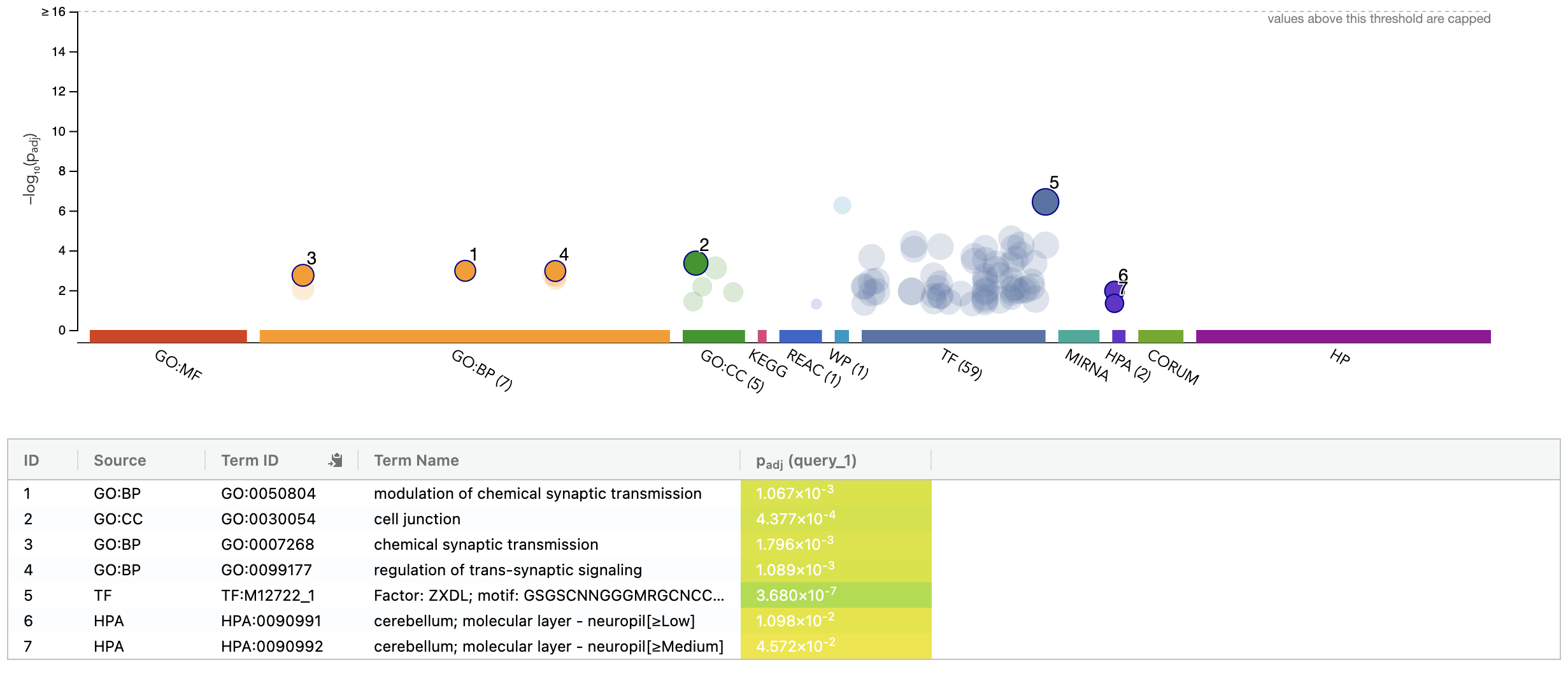
- Try querying with the top 100 HBR over-expressed genes using: g:Profiler
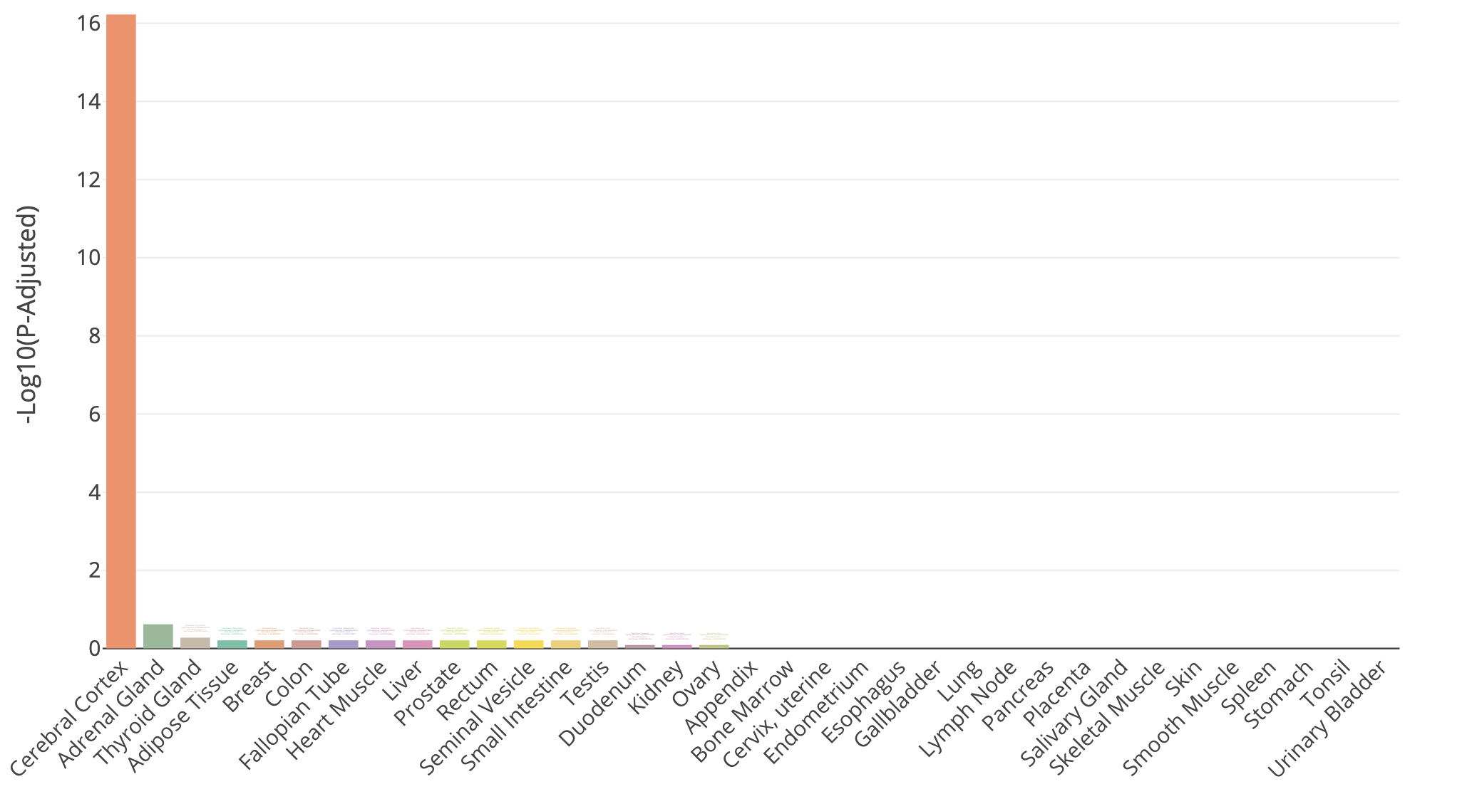
- Try querying with the top 100 HBR over-expressed genes using: TissueEnrich. Use the Tissue Enrichment tool. This tool also requires a Background Gene List. Use all genes in
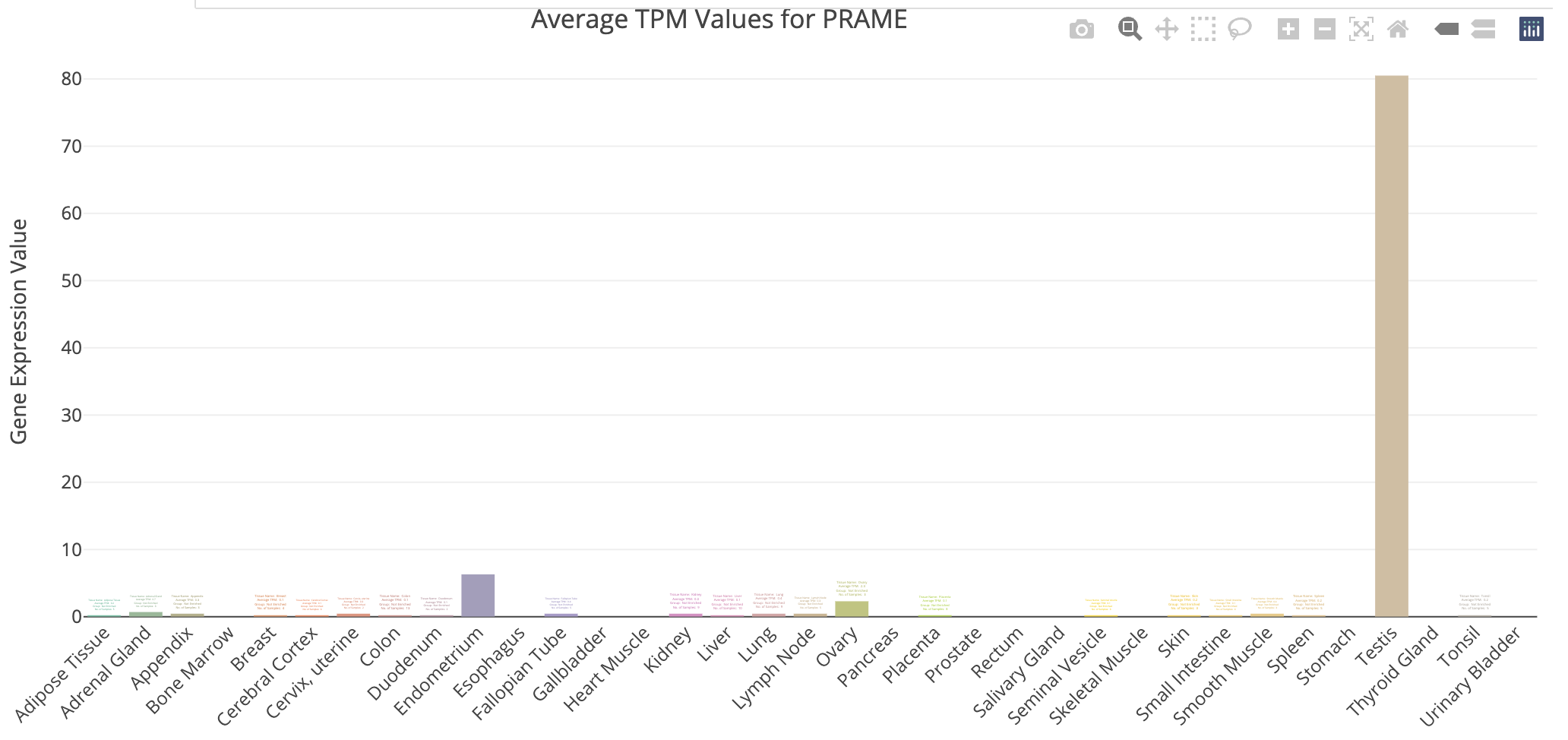
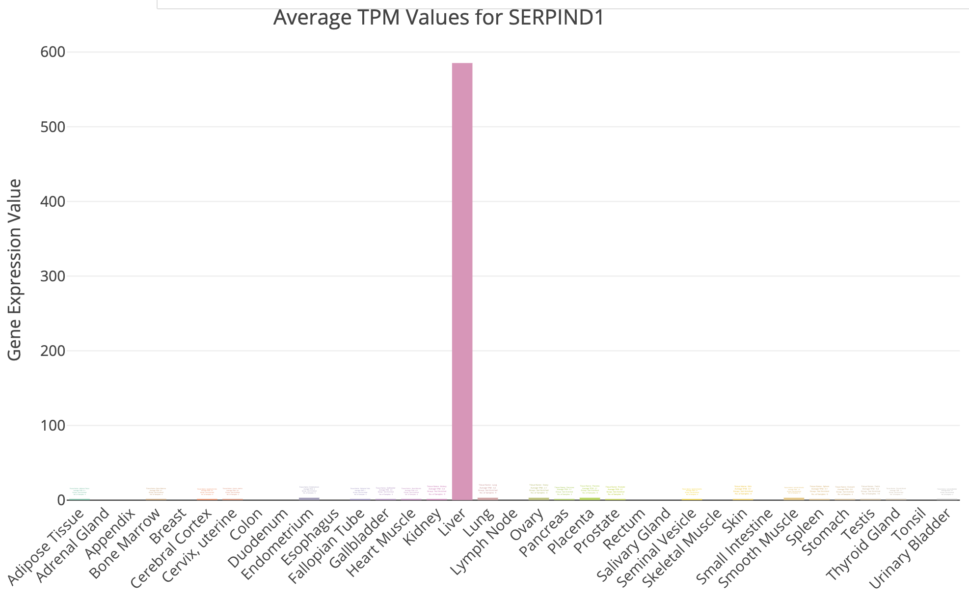
DE_all_genes_DESeq2.tsvfor this purpose. You can also manually explore some individual genes over-expressed in UHR with the Tissue-Specific Genes tool. For example, try PRAME and SERPIND1, two of the top UHR genes.
g:Profiler example result
TissueEnrich summary for top 100 HBR over-expressed genes
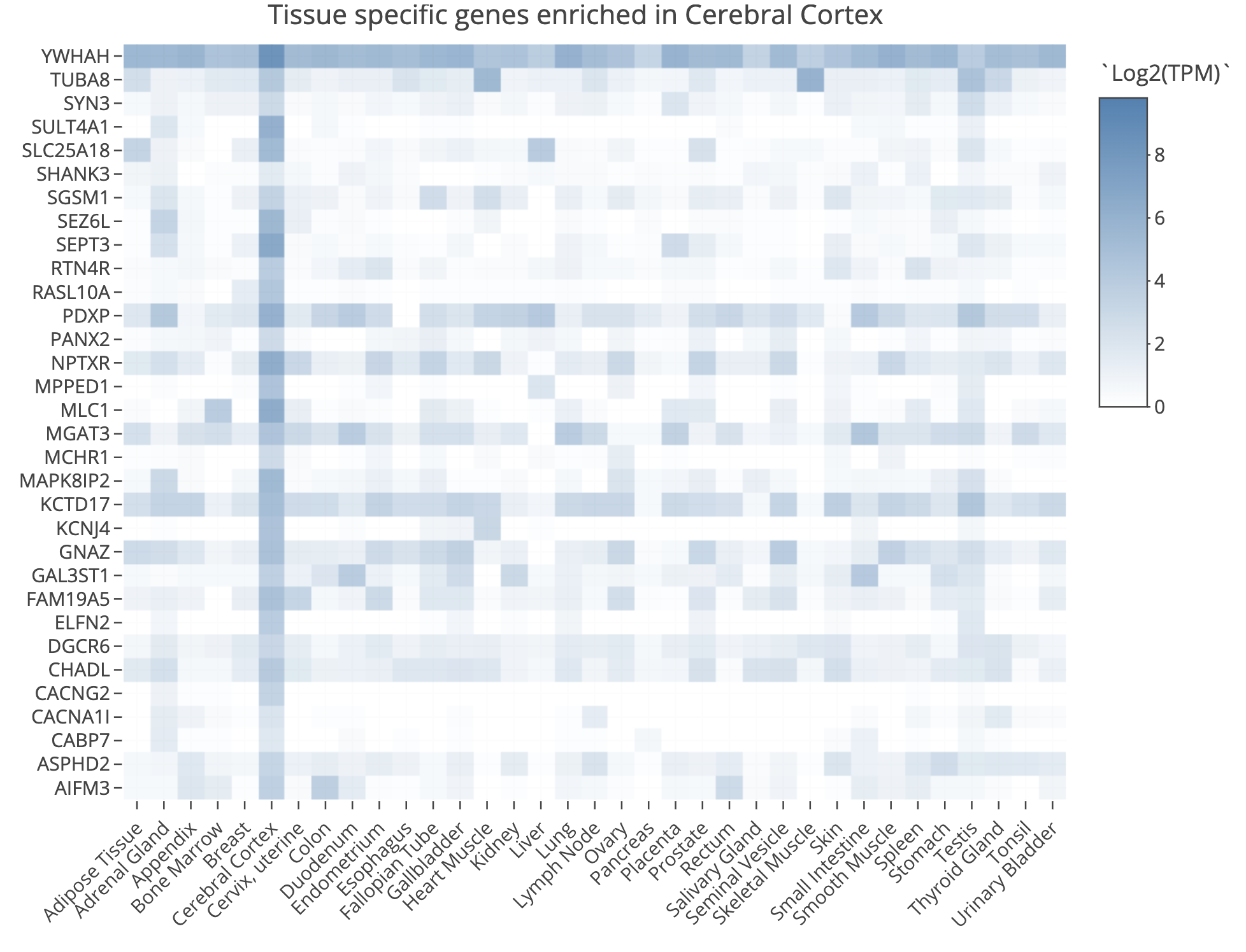
TissueEnrich result for Cerebral Cortex tissue
TissueEnrich example for UHR over-expressed gene: PRAME
TissueEnrich example for UHR over-expressed gene: SERPIND1
Does all of this make sense when we think about the makeup of the HBR and UHR samples? Refer back to the description of the samples.