Posts
My thoughts and ideas
Welcome to the blog
My thoughts and ideas
Introduction to bioinformatics for RNA sequence analysis
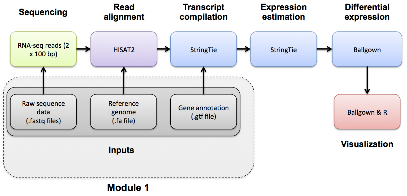
If you would like a refresher on common file formats such as FASTA, FASTQ, and GTF files, we have made a mini lecture briefly covering these.
In this example analysis we will use the human GRCh38 version of the genome from Ensembl. Furthermore, we are actually going to perform the analysis using only a single chromosome (chr22) and the ERCC spike-in to make it run faster.
First we will create the necessary working directory.
cd $RNA_HOME
echo $RNA_REFS_DIR
mkdir -p $RNA_REFS_DIR
The complete data from which these files were obtained can be found at: ftp://ftp.ensembl.org/pub/release-86/fasta/homo_sapiens/dna/. You could use wget to download the Homo_sapiens.GRCh38.dna_sm.primary_assembly.fa.gz file, then unzip/untar.
We have prepared this simplified reference for you. It contains chr22 (and ERCC transcript) fasta files in both a single combined file and individual files. Download the reference genome file to the rnaseq working directory
cd $RNA_REFS_DIR
wget https://genomedata.org/rnaseq-tutorial/fasta/GRCh38/chr22_with_ERCC92.fa
# if this is taking too long, you can find it cached under the CourseData directory in the AWS instance:
# cp ~/CourseData/module02_referenceGenomes/chr22_with_ERCC92.fa .
ls
View the first 10 lines of this file. Why does it look like this?
head chr22_with_ERCC92.fa
How many lines and characters are in this file? How long is this chromosome (in bases and Mbp)?
wc chr22_with_ERCC92.fa
View 10 lines from approximately the middle of this file. What is the significance of the upper and lower case characters?
head -n 425000 chr22_with_ERCC92.fa | tail
What is the count of each base in the entire reference genome file (skipping the header lines for each sequence)?
cat chr22_with_ERCC92.fa | grep -v ">" | perl -ne 'chomp $_; $bases{$_}++ for split //; if (eof){print "$_ $bases{$_}\n" for sort keys %bases}'
Note: Instead of the above, you might consider getting reference genomes and associated annotations from UCSC. e.g., UCSC GRCh38 download.
Wherever you get them from, remember that the names of your reference sequences (chromosomes) must those matched in your annotation gtf files (described in the next section).
View a list of all sequences in our reference genome fasta file.
grep ">" chr22_with_ERCC92.fa
Take a closer look at the command above that counts the occurrence of each nucleotide base in our chr22 reference sequence. Note that for even a seemingly simple question, commands can become quite complex. In that approach, a combination of Unix commands, pipes, and the scripting language Perl are used to answer the question. In bioinformatics, generally this kind of scripting comes up before too long, because you have an analysis question that is so specific there is no out of the box tool available. Or an existing tool will give perform a much more complex and involved analysis than needed to answer a very focused question.
In Unix there are usually many ways to solve the same problem. Perl as a language has mostly fallen out of favor. This kind of simple text parsing problem is one area it perhaps still remains relevant. Let’s benchmark the run time of the previous approach and constrast with several alternatives that do not rely on Perl.
Each of the following gives exactly the same answer. time is used to measure the run time of each alternative. Each starts by using cat to dump the file to standard out and then using grep to remove the header lines starting with “>”. Each ends with column -t to make the output line up consistently.
#1. The Perl approach. This command removes the end of line character with chomp, then it splits each line into an array of individual characters, amd it creates a data structure called a hash to store counts of each letter on each line. Once the end of the file is reached it prints out the contents of this data structure in order.
time cat chr22_with_ERCC92.fa | grep -v ">" | perl -ne 'chomp $_; $bases{$_}++ for split //; if (eof){print "$bases{$_} $_\n" for sort keys %bases}' | column -t

#2. The Awk approach. Awk is an alternative scripting language include in most linux distributions. This command is conceptually very similar to the Perl approach but with a different syntax. A for loop is used to iterate over each character until the end ("NF") is reached. Again the counts for each letter are stored in a simple data structure and once the end of the file is reach the results are printed.
time cat chr22_with_ERCC92.fa | grep -v ">" | awk '{for (i=1; i<=NF; i++){a[$i]++}}END{for (i in a){print a[i], i}}' FS= - | sort -k 2 | column -t

#3. The Sed approach. Sed is an alternative scripting language. "tr" is used to remove newline characters. Then sed is used simply to split each character onto its own line, effectively creating a file with millions of lines. Then unix sort and uniq are used to produce counts of each unique character, and sort is used to order the results consistently with the previous approaches.
time cat chr22_with_ERCC92.fa | grep -v ">" | tr -d '\n' | sed 's/\(.\)/\1\n/g'  - | sort | uniq -c | sort -k 2 | column -t

#4. The grep appoach. The "-o" option of grep splits each match onto a line which we then use to get a count. The "-i" option makes the matching work for upper/lower case. The "-P" option allows us to use Perl style regular expressions with Greg.
time cat chr22_with_ERCC92.fa | grep -v ">" | grep -i -o -P "a|c|g|t|y|n" | sort | uniq -c

#5. Finally, the simplest/shortest approach that leverages the unix fold command to split each character onto its own line as in the Sed example.
time cat chr22_with_ERCC92.fa | grep -v ">" | fold -w1 | sort | uniq -c | column -t
Which method is fastest? Why are the first two approaches so much faster than the others?
Assignment: Use a commandline scripting approach of your choice to further examine our chr22 reference genome file and answer the following questions.
Questions:
Hint: Each question can be tackled using approaches similar to those above, using the file ‘chr22_with_ERCC92.fa’ as a starting point. Hint: To make things simpler, first produce a file with only the chr22 sequence. Hint: Remember that repetitive elements in the sequence are represented in lower case
Solution: When you are ready you can check your approach against the Solutions.