Welcome to the blog

Posts

My thoughts and ideas

IGV | Griffith Lab

RNA-seq Bioinformatics

Introduction to bioinformatics for RNA sequence analysis

IGV


Introduction

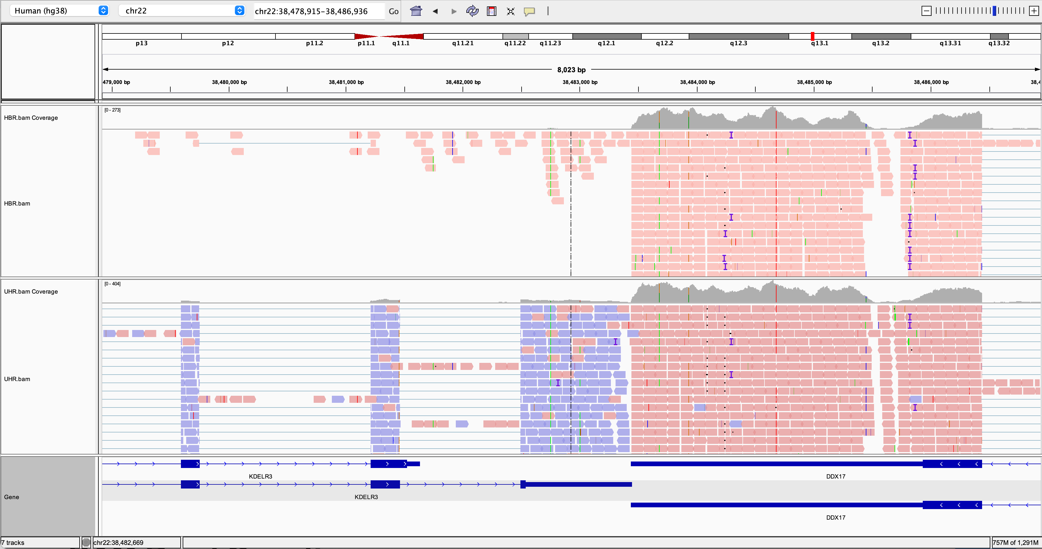
Description of the lab Welcome to the lab for Genome Visualization! This lab will introduce you to the Integrative Genomics Viewer, one of the most popular visualization tools for High Throughput Sequencing (HTS) data.

Lecture files that accompany this tutorial:

After this lab, you will be able to:

  • Visualize a variety of genomic data
  • Quickly navigate around the genome
  • Visualize read alignments
  • Validate SNP/SNV calls and structural re-arrangements by eye

Things to know before you start:

  • The lab may take between 1-2 hours, depending on your familiarity with genome browsing. Do not worry if you do not complete the lab. It will remain available to review later.

  • There are a few thought-provoking Questions or Notes pertaining to sections of the lab. These are optional, and may take more time, but are meant to help you better understand the visualizations you are seeing. These questions will be denoted by boxes, as follows: Question(s):

Thought-provoking question goes here.`

Requirements

  • Integrative Genomics Viewer

  • Ability to run Java

  • Note that while most tutorials in this course are performed on the cloud, IGV will always be run on your local machine

  • Note a version of this tutorial can also be performed directly in your web browser at sandbox.bio IGV Intro.

Compatibility

This tutorial was most recently updated for IGV v2.16.2, which is available on the IGV Download page. It is recommended that you use this version. Most other recent versions will work but their may be slight differences.

Data Set for IGV

We will be using publicly available Illumina sequence data from the HCC1143 cell line. The HCC1143 cell line was generated from a 52 year old caucasian woman with breast cancer. Additional information on this cell line can be found here: HCC1143 (tumor, TNM stage IIA, grade 3, primary ductal carcinoma) and HCC1143/BL (matched normal EBV transformed lymphoblast cell line).


Visualization Part 1: Getting familiar with IGV

We will be visualizing read alignments using IGV, a popular visualization tool for HTS data.

First, lets familiarize ourselves with it.

Get familiar with the interface

Load a Genome and some Data Tracks

By default, IGV loads the Human GRCh38/hg38 reference genome. If you work with another version of the human genome, or another organism altogether, you can change the genome by clicking the drop down menu in the upper-left. For this lab, we will be using Human GRCh37/hg19.

We will also load additional tracks from Server using (File -> Load from Server...):

  • Ensembl Genes (or your favourite source of gene annotations)
  • GC Percentage
  • dbSNP 1.4.7

Load hg19 genome and additional data tracks

Load hg19 genome and additional data tracks

You should see listing of chromosomes in this reference genome. Choose 1, for chromosome 1.

Chromosome chooser

Chromosome chooser

Navigate to chr1:10,000-11,000 by entering this into the location field (in the top-left corner of the interface) and clicking Go. This shows a window of chromosome 1 that is 1,000 base pairs wide and beginning at position 10,000.

Navigition using Location text field. Sequence displayed as thin coloured rectangles.

Navigition using Location text field. Sequence displayed as thin coloured rectangles.

IGV displays the sequence of letters in a genome as a sequence of colours (e.g. A = green, C = blue, etc.). This makes repetitive sequences, like the ones found at the start of this region, easy to identify. Zoom in a bit more using the + button to see the individual bases of the reference genome sequence.

You can navigate to a gene of interest by typing it in the same box the genomic coordinates are in and pressing Enter/Return. Try it for your favourite gene, or BRCA1 if you can not decide.

Gene model

Gene model

Genes are represented as lines and boxes. Lines represent intronic regions, and boxes represent exonic regions. The arrows indicate the direction/strand of transcription for the gene. When an exon box become narrower in height, this indicates a UTR.

When loaded, tracks are stacked on top of each other. You can identify which track is which by consulting the label to the left of each track.

Region Lists

Sometimes, it is really useful to save where you are, or to load regions of interest. For this purpose, there is a Region Navigator in IGV. To access it, click Regions > Region Navigator. While you browse around the genome, you can save some bookmarks by pressing the Add button at any time.

Bookmarks in IGV

Bookmarks in IGV

Loading Read Alignments

We will be using the breast cancer cell line HCC1143 to visualize alignments. For speed, only a small portion of chr21 will be loaded (19M:20M).

HCC1143 Alignments to hg19:

Copy the files to your local drive, and in IGV choose File > Load from File..., select the bam file, and click OK. Note that the bam and index files must be in the same directory for IGV to load these properly.

Load BAM track from File

Load BAM track from File

Visualizing read alignments

Navigate to a narrow window on chromosome 21: chr21:19,480,041-19,480,386.

To start our exploration, right click on the read alignment track, and select the following options:

  • Sort alignments by -> start location
  • Group alignments by -> pair orientation

Experiment with the various settings by right clicking the read alignment track and toggling the options. Think about which would be best for specific tasks (e.g. quality control, SNP calling, CNV finding).

Changing how read alignments are sorted, grouped, and colored

Changing how read alignments are sorted, grouped, and colored

You will see reads represented by grey or white bars stacked on top of each other, where they were aligned to the reference genome. The reads are pointed to indicate their orientation (i.e. the strand on which they are mapped). Mouse over any read and notice that a lot of information is available. To toggle read display from hover to click, select the yellow box and change the setting.

Changing how read information is shown (i.e. on hover, click, never)

Changing how read information is shown (i.e. on hover, click, never)

Once you select a read, you will learn what many of these metrics mean, and how to use them to assess the quality of your datasets. At each base that the read sequence mismatches the reference, the colour of the base represents the letter that exists in the read (using the same colour legend used for displaying the reference).

Viewing read information for a single aligned read

Viewing read information for a single aligned read


Visualization Part 2: Inspecting SNPs, SNVs, and SVs

In this section we will be looking in detail at 8 positions in the genome, and determining whether they represent real events or artifacts.

Two neighbouring SNPs

  • Navigate to region chr21:19,479,237-19,479,814

  • Note two heterozygous variants, one corresponds to a known dbSNP (G/T on the right) the other does not (C/T on the left)

  • Zoom in and center on the C/T SNV on the left, sort by base (window chr21:19,479,321 is the SNV position)

  • Sort alignments by base

  • Color alignments by read strand

Example1. Good quality SNVs/SNPs

Example1. Good quality SNVs/SNPs

Notes:

  • High base qualities in all reads except one (where the alt allele is the last base of the read)
  • Good mapping quality of reads, no strand bias, allele frequency consistent with heterozygous mutation

Question(s):

* What does *Shade base by quality* do? How might this be helpful?
* How does Color by *read strand* help?

Homopolymer region with indel

Navigate to position chr21:19,518,412-19,518,497

Example 2a

  • Group alignments by read strand
  • Center on the A within the homopolymer run (chr21:19,518,470), and Sort alignments by -> base

Example 2a

Example 2b

  • Center on the one base deletion (chr21:19,518,452), and Sort alignments by -> base

Example 2b

Notes:

  • The alt allele is either a deletion or insertion of one or two Ts
  • The remaining bases are mismatched, because the alignment is now out of sync

Coverage by GC

Navigate to position chr21:19,611,925-19,631,555. Note that the range contains areas where coverage drops to zero in a few places.

Example 3

  • Use Collapsed view
  • Color alignments by -> insert size and pair orientation
  • Group alignments by -> none
  • Load GC track (if not already loaded above)
  • See concordance of coverage with GC content

Example 3

Question:

* Why are there blue and red reads throughout the alignments?

Heterozygous SNPs on different alleles

Navigate to region chr21:19,666,833-19,667,007

Example 4

  • Sort by base (at position chr21:19,666,901)

Example 4

Note:

  • There is no linkage between alleles for these two SNPs because reads covering both only contain one or the other

Low mapping quality

Navigate to region chr21:19,800,320-19,818,162

  • Load repeat track (File -> Load from server...)

Load repeats

Load repeats

Example 5

Example 5

Notes:

  • Mapping quality plunges in all reads (white instead of grey). Once we load repeat elements, we see that there are two LINE elements that cause this.

Homozygous deletion

Navigate to region chr21:19,324,469-19,331,468

Example 6

  • Turn on View as Pairs and Expanded view
  • Use Color alignments by -> insert size and pair orientation
  • Sort reads by insert size
  • Click on a red read pair to pull up information on alignments

Example 6

Notes:

  • Typical insert size of read pair in the vicinity: 350bp
  • Insert size of red read pairs: 2,875bp
  • This corresponds to a homozygous deletion of 2.5kb

Mis-alignment

Navigate to region chr21:19,102,154-19,103,108

Example 7

Example 7

Notes:

  • This is a position where AluY element causes mis-alignment.
  • Misaligned reads have mismatches to the reference and well-aligned reads have partners on other chromosomes where additional ALuY elements are encoded.
  • Zoom out until you can clearly see the contrast between the difficult alignment region (corresponding to an AluY) and regions with clean alignments on either side

Translocation

Navigate to region chr21:19,089,694-19,095,362

Example 8

  • Expanded view
  • Group alignments by -> pair orientation
  • Color alignments by -> insert size and pair orientation

Example 8

Notes:

  • Many reads with mismatches to reference
  • Read pairs in RL pattern (instead of LR pattern)
  • Region is flanked by reads with poor mapping quality (white instead of grey)
  • Presence of reads with pairs on other chromosomes (coloured reads at the bottom when scrolling down)

Visualization Part 3: Automating Tasks in IGV

We can use the Tools menu to invoke running a batch script. Batch scripts are described on the IGV website:

Download the batch script and the attribute file for our dataset:

Now run the file from the Tools menu:

Automation

Automation

Notes:

  • This script will navigate automatically to each location in the lab
  • A screenshot will be taken and saved to the screenshots directory specified

Contributors/acknowledgements

Malachi Griffith, Sorana Morrissy, Jim Robinson, Ben Ainscough, Jason Walker, Obi Griffith

Alignment | Griffith Lab

RNA-seq Bioinformatics

Introduction to bioinformatics for RNA sequence analysis

Alignment

Alignment mini lecture

If you would like a refresher on alignment, we have created an alignment mini lecture.

We have also provided a mini lectures describing the differences between alignment, assembly, and pseudoalignment and describing sam, bam, and bed file formats.

HISAT2 alignment

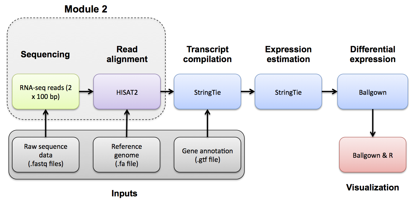
Perform alignments with HISAT2 to the genome and transcriptome.

First, begin by making the appropriate output directory for our alignment results.

echo $RNA_ALIGN_DIR
mkdir -p $RNA_ALIGN_DIR
cd $RNA_ALIGN_DIR

HISAT2 uses a graph-based alignment and has succeeded HISAT and TOPHAT2. The output of this step will be a SAM/BAM file for each data set.

Refer to HISAT2 manual for a more detailed explanation:

HISAT2 basic usage:

#hisat2 [options]* -x <ht2-idx> {-1 <m1> -2 <m2> | -U <r> | --sra-acc <SRA accession number>} [-S <sam>]

Extra options specified below:

hisat2 -p 4 --rg-id=UHR_Rep1 --rg SM:UHR --rg LB:UHR_Rep1_ERCC-Mix1 --rg PL:ILLUMINA --rg PU:CXX1234-ACTGAC.1 -x $RNA_REF_INDEX --dta --rna-strandness RF -1 $RNA_DATA_DIR/UHR_Rep1_ERCC-Mix1_Build37-ErccTranscripts-chr22.read1.fastq.gz -2 $RNA_DATA_DIR/UHR_Rep1_ERCC-Mix1_Build37-ErccTranscripts-chr22.read2.fastq.gz -S ./UHR_Rep1.sam
hisat2 -p 4 --rg-id=UHR_Rep2 --rg SM:UHR --rg LB:UHR_Rep2_ERCC-Mix1 --rg PL:ILLUMINA --rg PU:CXX1234-TGACAC.1 -x $RNA_REF_INDEX --dta --rna-strandness RF -1 $RNA_DATA_DIR/UHR_Rep2_ERCC-Mix1_Build37-ErccTranscripts-chr22.read1.fastq.gz -2 $RNA_DATA_DIR/UHR_Rep2_ERCC-Mix1_Build37-ErccTranscripts-chr22.read2.fastq.gz -S ./UHR_Rep2.sam
hisat2 -p 4 --rg-id=UHR_Rep3 --rg SM:UHR --rg LB:UHR_Rep3_ERCC-Mix1 --rg PL:ILLUMINA --rg PU:CXX1234-CTGACA.1 -x $RNA_REF_INDEX --dta --rna-strandness RF -1 $RNA_DATA_DIR/UHR_Rep3_ERCC-Mix1_Build37-ErccTranscripts-chr22.read1.fastq.gz -2 $RNA_DATA_DIR/UHR_Rep3_ERCC-Mix1_Build37-ErccTranscripts-chr22.read2.fastq.gz -S ./UHR_Rep3.sam

hisat2 -p 4 --rg-id=HBR_Rep1 --rg SM:HBR --rg LB:HBR_Rep1_ERCC-Mix2 --rg PL:ILLUMINA --rg PU:CXX1234-TGACAC.1 -x $RNA_REF_INDEX --dta --rna-strandness RF -1 $RNA_DATA_DIR/HBR_Rep1_ERCC-Mix2_Build37-ErccTranscripts-chr22.read1.fastq.gz -2 $RNA_DATA_DIR/HBR_Rep1_ERCC-Mix2_Build37-ErccTranscripts-chr22.read2.fastq.gz -S ./HBR_Rep1.sam
hisat2 -p 4 --rg-id=HBR_Rep2 --rg SM:HBR --rg LB:HBR_Rep2_ERCC-Mix2 --rg PL:ILLUMINA --rg PU:CXX1234-GACACT.1 -x $RNA_REF_INDEX --dta --rna-strandness RF -1 $RNA_DATA_DIR/HBR_Rep2_ERCC-Mix2_Build37-ErccTranscripts-chr22.read1.fastq.gz -2 $RNA_DATA_DIR/HBR_Rep2_ERCC-Mix2_Build37-ErccTranscripts-chr22.read2.fastq.gz -S ./HBR_Rep2.sam
hisat2 -p 4 --rg-id=HBR_Rep3 --rg SM:HBR --rg LB:HBR_Rep3_ERCC-Mix2 --rg PL:ILLUMINA --rg PU:CXX1234-ACACTG.1 -x $RNA_REF_INDEX --dta --rna-strandness RF -1 $RNA_DATA_DIR/HBR_Rep3_ERCC-Mix2_Build37-ErccTranscripts-chr22.read1.fastq.gz -2 $RNA_DATA_DIR/HBR_Rep3_ERCC-Mix2_Build37-ErccTranscripts-chr22.read2.fastq.gz -S ./HBR_Rep3.sam

Note: in the above alignments, we are treating each library as an independent data set. If you had multiple lanes of data for a single library, you could align them all together in one HISAT2 command. Similarly you might combine technical replicates into a single alignment run (perhaps after examining them and removing outliers…). To combine multiple lanes, you would provide all the read1 files as a comma separated list for the ‘-1’ input argument, and then all read2 files as a comma separated list for the ‘-2’ input argument, (where both lists have the same order) : You can also use samtools merge to combine bam files after alignment. This is the approach we will take.

HISAT2 Alignment Summary HISAT2 generates a summary of the alignments printed to the terminal. Notice the number of total reads, reads aligned and various metrics regarding how the reads aligned to the reference.

SAM to BAM Conversion Convert HISAT2 sam files to bam files and sort by aligned position

samtools sort -@ 4 -o UHR_Rep1.bam UHR_Rep1.sam
samtools sort -@ 4 -o UHR_Rep2.bam UHR_Rep2.sam
samtools sort -@ 4 -o UHR_Rep3.bam UHR_Rep3.sam
samtools sort -@ 4 -o HBR_Rep1.bam HBR_Rep1.sam
samtools sort -@ 4 -o HBR_Rep2.bam HBR_Rep2.sam
samtools sort -@ 4 -o HBR_Rep3.bam HBR_Rep3.sam

Merge HISAT2 BAM files

Make a single BAM file combining all UHR data and another for all HBR data. Note: This could be done in several ways such as ‘samtools merge’, ‘bamtools merge’, or using picard-tools (see below). We chose the third method because it did the best job at merging the bam header information. NOTE: sambamba also retains header info.

cd $RNA_HOME/alignments/hisat2
java -Xmx2g -jar $PICARD MergeSamFiles -OUTPUT UHR.bam -INPUT UHR_Rep1.bam -INPUT UHR_Rep2.bam -INPUT UHR_Rep3.bam
java -Xmx2g -jar $PICARD MergeSamFiles -OUTPUT HBR.bam -INPUT HBR_Rep1.bam -INPUT HBR_Rep2.bam -INPUT HBR_Rep3.bam

Count the alignment (BAM) files to make sure all were created successfully (you should have 8 total)

ls -l *.bam | wc -l
ls -l *.bam


PRACTICAL EXERCISE 6

Assignment: Perform some alignments on additional read data sets. Align the reads using the skills you learned above. Try using the HISAT2 aligner. Also practice converting SAM to BAM files, and merging BAM files.

Hint: Do this analysis on the additional data and in the separate working directory called ‘practice’ that you created in Practical Exercise 3. Questions

What is the difference between a .sam and .bam file? If you sorted the resulting BAM file as we did above, is the result sorted by read name? Or position? Which columns of the BAM file can be viewed to determine the style of sorting? What command can you use to view only the BAM header?

Solution: When you are ready you can check your approach against the Solutions.