Posts
My thoughts and ideas
Welcome to the blog
My thoughts and ideas
Introduction to bioinformatics for RNA sequence analysis
If you would like a refresher on Kallisto, we have made a mini lecture briefly covering the topic. We have also made a mini lecture describing the differences between alignment, assembly, and pseudoalignment.
For more information on Kallisto, refer to the Kallisto project page, the Kallisto manual page and the Kallisto manuscript.
Note that we already have fasta sequences for the reference genome sequence from earlier in the RNA-seq tutorial. However, Kallisto works directly on target cDNA/transcript sequences. Remember also that we have transcript models for genes on chromosome 22. These transcript models were downloaded from Ensembl in GTF format. This GTF contains a description of the coordinates of exons that make up each transcript but it does not contain the transcript sequences themselves. So currently we do not have transcript sequences needed by Kallisto. There are many places we could obtain these transcript sequences. For example, we could download them directly in Fasta format from the Ensembl FTP site.
To allow us to compare Kallisto results to expression results from StringTie, we will create a custom Fasta file that corresponds to the transcripts we used for the StringTie analysis. How can we obtain these transcript sequences in Fasta format?
We could download the complete fasta transcript database for human and pull out only those for genes on chromosome 22.
We can also use BedTools to create a transcripts fastq file from our transcript GTF file. Note that previously in the alignment QC section we converted our transcript GTF file to the bed12 format needed for the following step. This approach is convenient because it will also include the sequences for the ERCC spike in controls, allowing us to generate Kallisto abundance estimates for those features as well. Use bedtools getfasta to create an Ensembl+ERCC92 transcripts fasta file as follows.
cd $RNA_HOME/refs
bedtools getfasta -fi chr22_with_ERCC92.fa -bed chr22_with_ERCC92.bed12 -s -split -name -fo chr22_ERCC92_transcripts.fa

# to see an explanation of the options used in this command:
bedtools getfasta
Note that we could have instead used a tool from tophat called gtf_to_fasta to generate the fasta sequence from our GTF file. HOWEVER, when this tool splices defined exons in our GTF together using the sequence in our reference genome FASTA file it does NOT reverse complement the genes expressed on the -ve strand. This is fine if you do NOT specify the strand option when running kallisto quant. BUT, if you intend to use the strand specific options, then all of your transcripts MUST be represented in the forward (5’->3’ direction). gtf_to_fasta does not have an option to create them this way. So you should use one of the approaches two described above. Either download a transcript file where all sequences are already represented in the correct forward orientation, OR use the getfasta strategy above on a bed12 version of your transcript GTF.
Use less to view the file chr22_ERCC92_transcripts.fa. Note that this file has messy transcript names. Use the following hairball Perl one-liner to tidy up the header line for each fasta sequence. This Perl expression looks complex but it is really just looking for header lines the FASTA file that match one of two patterns (those that have names like ERCC… and those that have regular Ensembl transcript names). To learn more about this kind of string matching/parsing, you can refer to the Perl regular expression documentation.
cd $RNA_HOME/refs
cat chr22_ERCC92_transcripts.fa | perl -ne 'if($_ =~/^\>\S+\:\:(ERCC\-\d+)\:.*/){print ">$1\n"}elsif ($_ =~/^\>(\S+)\:\:.*/){print ">$1\n"}else{print $_}' > chr22_ERCC92_transcripts.clean.fa
wc -l chr22_ERCC92_transcripts*.fa
View the resulting ‘clean’ file using less chr22_ERCC92_transcripts.clean.fa. View the end of this file use tail chr22_ERCC92_transcripts.clean.fa. Note that we have one fasta record for each Ensembl transcript on chromosome 22 and we have an additional fasta record for each ERCC spike-in sequence.
Create a list of all transcript IDs for later use:
cd $RNA_HOME/refs
cat chr22_ERCC92_transcripts.clean.fa | grep ">" | perl -ne '$_ =~ s/\>//; print $_' | sort | uniq > transcript_id_list.txt
Remember that Kallisto does not perform alignment or use a reference genome sequence. Instead it performs pseudoalignment to determine the compatibility of reads with targets (transcript sequences in this case). However, similar to alignment algorithms like Tophat or STAR, Kallisto requires an index to assess this compatibility efficiently and quickly.
cd $RNA_HOME/refs
mkdir kallisto
cd kallisto
kallisto index --index=chr22_ERCC92_transcripts_kallisto_index ../chr22_ERCC92_transcripts.clean.fa
As we did with StringTie and HT-Seq we will generate transcript abundances for each of our demonstration samples using Kallisto.
echo $RNA_DATA_DIR

cd $RNA_HOME/expression/
mkdir kallisto
cd kallisto

kallisto quant --rf-stranded --index=$RNA_HOME/refs/kallisto/chr22_ERCC92_transcripts_kallisto_index --output-dir=UHR_Rep1_ERCC-Mix1 --threads=4 --plaintext $RNA_DATA_DIR/UHR_Rep1_ERCC-Mix1_Build37-ErccTranscripts-chr22.read1.fastq.gz $RNA_DATA_DIR/UHR_Rep1_ERCC-Mix1_Build37-ErccTranscripts-chr22.read2.fastq.gz
kallisto quant --rf-stranded --index=$RNA_HOME/refs/kallisto/chr22_ERCC92_transcripts_kallisto_index --output-dir=UHR_Rep2_ERCC-Mix1 --threads=4 --plaintext $RNA_DATA_DIR/UHR_Rep2_ERCC-Mix1_Build37-ErccTranscripts-chr22.read1.fastq.gz $RNA_DATA_DIR/UHR_Rep2_ERCC-Mix1_Build37-ErccTranscripts-chr22.read2.fastq.gz
kallisto quant --rf-stranded --index=$RNA_HOME/refs/kallisto/chr22_ERCC92_transcripts_kallisto_index --output-dir=UHR_Rep3_ERCC-Mix1 --threads=4 --plaintext $RNA_DATA_DIR/UHR_Rep3_ERCC-Mix1_Build37-ErccTranscripts-chr22.read1.fastq.gz $RNA_DATA_DIR/UHR_Rep3_ERCC-Mix1_Build37-ErccTranscripts-chr22.read2.fastq.gz

kallisto quant --rf-stranded --index=$RNA_HOME/refs/kallisto/chr22_ERCC92_transcripts_kallisto_index --output-dir=HBR_Rep1_ERCC-Mix2 --threads=4 --plaintext $RNA_DATA_DIR/HBR_Rep1_ERCC-Mix2_Build37-ErccTranscripts-chr22.read1.fastq.gz $RNA_DATA_DIR/HBR_Rep1_ERCC-Mix2_Build37-ErccTranscripts-chr22.read2.fastq.gz
kallisto quant --rf-stranded --index=$RNA_HOME/refs/kallisto/chr22_ERCC92_transcripts_kallisto_index --output-dir=HBR_Rep2_ERCC-Mix2 --threads=4 --plaintext $RNA_DATA_DIR/HBR_Rep2_ERCC-Mix2_Build37-ErccTranscripts-chr22.read1.fastq.gz $RNA_DATA_DIR/HBR_Rep2_ERCC-Mix2_Build37-ErccTranscripts-chr22.read2.fastq.gz
kallisto quant --rf-stranded --index=$RNA_HOME/refs/kallisto/chr22_ERCC92_transcripts_kallisto_index --output-dir=HBR_Rep3_ERCC-Mix2 --threads=4 --plaintext $RNA_DATA_DIR/HBR_Rep3_ERCC-Mix2_Build37-ErccTranscripts-chr22.read1.fastq.gz $RNA_DATA_DIR/HBR_Rep3_ERCC-Mix2_Build37-ErccTranscripts-chr22.read2.fastq.gz
Create a single TSV file that has the TPM abundance estimates for all six samples.
cd $RNA_HOME/expression/kallisto
paste */abundance.tsv | cut -f 1,2,5,10,15,20,25,30 > transcript_tpms_all_samples.tsv
ls -1 */abundance.tsv | perl -ne 'chomp $_; if ($_ =~ /(\S+)\/abundance\.tsv/){print "\t$1"}' | perl -ne 'print "target_id\tlength$_\n"' > header.tsv
cat header.tsv transcript_tpms_all_samples.tsv | grep -v "tpm" > transcript_tpms_all_samples.tsv2
mv transcript_tpms_all_samples.tsv2 transcript_tpms_all_samples.tsv
rm -f header.tsv
Take a look at the final kallisto result file we created:
head transcript_tpms_all_samples.tsv
tail transcript_tpms_all_samples.tsv
Note that if you have stranded RNA-seq data and you use the stranded analysis option, it is important to choose the correction option. Examine what happens if you specify no strand as done above and compare to use of --fr-stranded and --rf-stranded.
cd $RNA_HOME/expression/kallisto
mkdir strand_option_test
cd strand_option_test

kallisto quant --index=$RNA_HOME/refs/kallisto/chr22_ERCC92_transcripts_kallisto_index --output-dir=UHR_Rep1_ERCC-Mix1_No-Strand --threads=4 --plaintext $RNA_DATA_DIR/UHR_Rep1_ERCC-Mix1_Build37-ErccTranscripts-chr22.read1.fastq.gz $RNA_DATA_DIR/UHR_Rep1_ERCC-Mix1_Build37-ErccTranscripts-chr22.read2.fastq.gz
kallisto quant --rf-stranded --index=$RNA_HOME/refs/kallisto/chr22_ERCC92_transcripts_kallisto_index --output-dir=UHR_Rep1_ERCC-Mix1_RF-Stranded --threads=4 --plaintext $RNA_DATA_DIR/UHR_Rep1_ERCC-Mix1_Build37-ErccTranscripts-chr22.read1.fastq.gz $RNA_DATA_DIR/UHR_Rep1_ERCC-Mix1_Build37-ErccTranscripts-chr22.read2.fastq.gz
kallisto quant --fr-stranded --index=$RNA_HOME/refs/kallisto/chr22_ERCC92_transcripts_kallisto_index --output-dir=UHR_Rep1_ERCC-Mix1_FR-Stranded --threads=4 --plaintext $RNA_DATA_DIR/UHR_Rep1_ERCC-Mix1_Build37-ErccTranscripts-chr22.read1.fastq.gz $RNA_DATA_DIR/UHR_Rep1_ERCC-Mix1_Build37-ErccTranscripts-chr22.read2.fastq.gz
Find a gene where the transcript expression estimates vary depending on the strand setting. Why would this be case? If you visualize our HISAT BAM alignments from the previous sections does this help us understand what is going on here? For this data, what is the correct strand setting?
Some example transcripts with values from all three modes:
grep ENST00000447898 */abundance.tsv
grep ENST00000434568 */abundance.tsv
grep ERCC-00171 */abundance.tsv
Create a convenient table of the results from using each mode
paste */abundance.tsv | cut -f 1,2,5,10,15 > transcript_tpms_strand-modes.tsv
ls -1 */abundance.tsv | perl -ne 'chomp $_; if ($_ =~ /(\S+)\/abundance\.tsv/){print "\t$1"}' | perl -ne 'print "target_id\tlength$_\n"' > header.tsv
cat header.tsv transcript_tpms_strand-modes.tsv | grep -v "tpm" > transcript_tpms_strand-modes.tsv2
mv transcript_tpms_strand-modes.tsv2 transcript_tpms_strand-modes.tsv
rm -f header.tsv
Use R to produce comparisons of the three modes:
cd $RNA_HOME/expression/kallisto/strand_option_test/
R
R code has been provided below. Run the R commands detailed in this script in your R session.
library(ggplot2)
library(cowplot)

# load input data
data <- read.delim("~/workspace/rnaseq/expression/kallisto/strand_option_test/transcript_tpms_strand-modes.tsv")

# log2 transform the data
FR_data = log2((data$UHR_Rep1_ERCC.Mix1_FR.Stranded) + 1)
RF_data = log2((data$UHR_Rep1_ERCC.Mix1_RF.Stranded) + 1)
unstranded_data = log2((data$UHR_Rep1_ERCC.Mix1_No.Strand) + 1)

# create scatterplots for each pairwise comparison of kallisto abundance estimates generated using each of the different kallisto strand modes
FR_vs_unstranded = ggplot(data, aes(x = FR_data, y = unstranded_data)) + geom_point(alpha = 0.1) + ggtitle('FR vs No Strand') + xlab('FR log2(expression + 1)') + ylab('No Strand log2(expression + 1)')
RF_vs_unstranded = ggplot(data, aes(x = RF_data, y = unstranded_data)) + geom_point(alpha = 0.1) + ggtitle('RF vs No Strand') + xlab('RF log2(expression + 1)') + ylab('No Strand log2(expression + 1)')
FR_vs_RF <- ggplot(data, aes(x = FR_data, y = RF_data)) + geom_point(alpha = 0.1) + ggtitle('FR vs RF') + xlab('FR log2(expression + 1)') + ylab('RF log2(expression + 1)')

# plot the set of comparisons as a multipanel figure
pdf(file = "Kallisto_Strand_Option_Comparisons.pdf")
plot_grid(FR_vs_unstranded, RF_vs_unstranded, FR_vs_RF, ncol = 1, nrow = 3)
dev.off()

#Quit R
quit(save="no")
Refer to this table, originally from our associated publication for the strand setting info for various tools. Note that since the UHR and HBR data were generated with the TruSeq Stranded Kit, the correct strand setting for kallisto is --rf-stranded.
How similar are the results we obtained from each approach?
We can compare the expression value for each Ensembl transcript from chromosome 22 as well as the ERCC spike in controls.
To do this comparison, we need to gather the expression estimates for each of our replicates from each approach. The Kallisto transcript results were neatly organized into a single file above. For Kallisto gene expression estimates, we will simply sum the TPM values for transcripts of the same gene. Though it is ‘apples-to-oranges’, we can also compare Kallisto and StringTie expression estimates to the raw read counts from HtSeq-Count (but only at the gene level in this case). The following R code will pull together the various expression matrix files we created in previous steps and create some visualizations to compare them (for both transcript and gene estimates).
First create the gene version of the Kallisto TPM matrix
cd $RNA_HOME/expression/kallisto
wget https://raw.githubusercontent.com/griffithlab/rnabio.org/master/assets/scripts/kallisto_gene_matrix.pl
chmod +x kallisto_gene_matrix.pl
./kallisto_gene_matrix.pl --gtf_file=$RNA_HOME/refs/chr22_with_ERCC92.gtf  --kallisto_transcript_matrix_in=transcript_tpms_all_samples.tsv --kallisto_transcript_matrix_out=gene_tpms_all_samples.tsv
column -t gene_tpms_all_samples.tsv | less -S
Now load files and summarize results from each approach in R
cd $RNA_HOME/expression
R
R code has been provided below. Run the R commands detailed in this script in your R session.
###R code###
#Load libraries
library(ggplot2)

#Set the base working dir from which to access the input files
working_dir = "~/workspace/rnaseq/expression"
setwd(working_dir)

#Load in expression matrix files from each expression method
htseq_gene_counts = read.table("htseq_counts/gene_read_counts_table_all_final.tsv", sep = "\t", header = TRUE, as.is = 1, row.names = 1)
stringtie_gene = read.table("stringtie/ref_only/gene_tpm_all_samples.tsv", sep = "\t", header = TRUE, as.is = 1, row.names = 1)
stringtie_tran = read.table("stringtie/ref_only/transcript_tpm_all_samples.tsv", sep = "\t", header = TRUE, as.is = 1, row.names = 1)
stringtie_gene_fpkm = read.table("stringtie/ref_only/gene_fpkm_all_samples.tsv", sep = "\t", header = TRUE, as.is = 1, row.names = 1)
stringtie_tran_fpkm = read.table("stringtie/ref_only/transcript_fpkm_all_samples.tsv", sep = "\t", header = TRUE, as.is = 1, row.names = 1)
kallisto_gene = read.table("kallisto/gene_tpms_all_samples.tsv", sep = "\t", header = TRUE, as.is = 1, row.names = 1)
kallisto_tran = read.table("kallisto/transcript_tpms_all_samples.tsv", sep = "\t", header = TRUE, as.is = 1, row.names = 1)

#Summarize the data.frames created
dim(htseq_gene_counts)
dim(stringtie_gene)
dim(stringtie_gene_fpkm)
dim(kallisto_gene)

dim(stringtie_tran)
dim(stringtie_tran_fpkm)
dim(kallisto_tran)

#Reorganize the data.frames for total consistency
kallisto_names = c("length", "HBR_Rep1", "HBR_Rep2", "HBR_Rep3", "UHR_Rep1", "UHR_Rep2", "UHR_Rep3")
names(kallisto_gene) = kallisto_names
names(kallisto_tran) = kallisto_names

sample_names = c("HBR_Rep1", "HBR_Rep2", "HBR_Rep3", "UHR_Rep1", "UHR_Rep2", "UHR_Rep3")
gene_names = row.names(kallisto_gene)
tran_names = row.names(kallisto_tran)

htseq_gene_counts = htseq_gene_counts[gene_names, sample_names]
stringtie_gene = stringtie_gene[gene_names, sample_names]
stringtie_gene_fpkm = stringtie_gene_fpkm[gene_names, sample_names]
kallisto_gene = kallisto_gene[gene_names, sample_names]
stringtie_tran = stringtie_tran[tran_names, sample_names]
stringtie_tran_fpkm = stringtie_tran_fpkm[tran_names, sample_names]
kallisto_tran = kallisto_tran[tran_names, sample_names]

#Take a look at the top of each data.frame
head(htseq_gene_counts)
head(stringtie_gene)
head(stringtie_gene_fpkm)
head(kallisto_gene)
head(stringtie_tran)
head(stringtie_tran_fpkm)
head(kallisto_tran)

#1. Plot kallisto gene TPMs vs stringtie gene TPMs - Pick HBR_Rep1 data arbitrarily
stabvar = 0.1
HBR1_gene_data = data.frame(kallisto_gene[,"HBR_Rep1"], stringtie_gene[,"HBR_Rep1"], htseq_gene_counts[,"HBR_Rep1"])
names(HBR1_gene_data) = c("kallisto", "stringtie", "htseq")
p1 = ggplot(HBR1_gene_data, aes(log2(kallisto + stabvar), log2(stringtie + stabvar)))
p1 = p1 + geom_point()
p1 = p1 + geom_point(aes(colour = log2(htseq+stabvar))) + scale_colour_gradient(low = "yellow", high = "red")
p1 = p1 + xlab("Kallisto TPM") + ylab("StringTie TPM") + labs(colour = "HtSeq Counts")
p1 = p1 + labs(title = "HBR1 GENE expression values [log2(value + 0.1) scaled]")

#2. Plot kallisto transcript TPMs vs stringtie transcript TPMs
# But now use color to indicate whether each data point corresponds to real transcripts vs. spike-in controls
HBR1_tran_data = data.frame(kallisto_tran[, "HBR_Rep1"], stringtie_tran[, "HBR_Rep1"])
names(HBR1_tran_data) = c("kallisto", "stringtie")
spikein_status=grepl("ERCC", tran_names)
p2 = ggplot(HBR1_tran_data, aes(log2(kallisto + stabvar), log2(stringtie + stabvar)))
p2 = p2 + geom_point()
p2 = p2 + geom_point(aes(colour = spikein_status))
p2 = p2 + xlab("Kallisto TPM") + ylab("StringTie TPM") + labs(colour = "SpikeIn Status")
p2 = p2 + labs(title = "HBR1 TRANSCRIPT expression values [log2(value + 0.1) scaled]")

#3. Plot stringtie transcript TPMs vs. stringtie transcript FPKMs - Pick HBR_Rep1 data arbitrarily
# Indicate with the points whether the data are real transcripts vs. spike-in controls
HBR1_tran_data2 = data.frame(stringtie_tran[,"HBR_Rep1"], stringtie_tran_fpkm[, "HBR_Rep1"])
names(HBR1_tran_data2) = c("stringtie_TPM", "stringtie_FPKM")
p3 = ggplot(HBR1_tran_data2, aes(log2(stringtie_TPM + stabvar), log2(stringtie_FPKM + stabvar)))
p3 = p3 + geom_point()
p3 = p3 + geom_point(aes(colour = spikein_status))
p3 = p3 + geom_abline(intercept = 0, slope = 1)
p3 = p3 + xlab("StringTie TPM") + ylab("StringTie FPKM") + labs(colour = "SpikeIn Status")
p3 = p3 + labs(title = "HBR1 transcript expression values [log2(value + 0.1) scaled]")

#Print out the plots created above and store in a single PDF file
pdf(file="Kallisto-StringTie-HTSeqCount_Comparisons.pdf")
print(p1)
print(p2)
print(p3)
dev.off()

#Quit R
quit(save="no")
The output file can be viewed in your browser at the following url. Note, you must replace YOUR_PUBLIC_IPv4_ADDRESS with your own amazon instance IP (e.g., 101.0.1.101)).
https://YOUR_PUBLIC_IPv4_ADDRESS/rnaseq/expression/Kallisto-StringTie-HTSeqCount_Comparisons.pdf
A file copy of the above R code can be found here.
Suppose we just want to quickly assess the presence of a particular class of genes only (e.g. ribosomal RNA genes). We can obtain these genes from an Ensembl GTF file. In the example below we will use our chromosome 22 GTF file for demonstration purposes. But in a ‘real world’ experiment you would use a GTF for all chromosomes. Once we have found GTF records for ribosomal RNA genes, we will create a fasta file that contains the sequences for these transcripts, and then index this sequence database for use with Kallisto.
cd $RNA_HOME/refs
grep rRNA $RNA_REF_GTF > chr22_rRNA.gtf

gtfToGenePred chr22_rRNA.gtf chr22_rRNA.genePred
genePredToBed chr22_rRNA.genePred chr22_rRNA.bed12
bedtools getfasta -fi $RNA_REF_FASTA -bed chr22_rRNA.bed12 -s -split -name -fo chr22_rRNA_transcripts.fa

cat chr22_rRNA_transcripts.fa | perl -ne 'if($_ =~/^\>\S+\:\:(ERCC\-\d+)\:.*/){print ">$1\n"}elsif ($_ =~/^\>(\S+)\:\:.*/){print ">$1\n"}else{print $_}' > chr22_rRNA_transcripts.clean.fa
cat chr22_rRNA_transcripts.clean.fa

cd $RNA_HOME/refs/kallisto
kallisto index --index=chr22_rRNA_transcripts_kallisto_index ../chr22_rRNA_transcripts.clean.fa
We can now use this index with Kallisto to assess the abundance of rRNA genes in a set of samples.
We will now use Sleuth perform a differential expression analysis on the full chr22 data set produced above. Sleuth is a companion tool that starts with the output of Kallisto, performs DE analysis, and helps you visualize the results. It is analagous to Ballgown that we used to perform DE and visualization of the StringTie results in earlier steps.
Regenerate the Kallisto results using the HDF5 format and 100 rounds of bootstrapping (both required for Sleuth to work).
cd $RNA_HOME/de
mkdir -p sleuth/input
mkdir -p sleuth/results
cd sleuth/input

kallisto quant --rf-stranded -b 100 --index=$RNA_HOME/refs/kallisto/chr22_ERCC92_transcripts_kallisto_index --output-dir=UHR_Rep1_ERCC-Mix1 --threads=4 $RNA_DATA_DIR/UHR_Rep1_ERCC-Mix1_Build37-ErccTranscripts-chr22.read1.fastq.gz $RNA_DATA_DIR/UHR_Rep1_ERCC-Mix1_Build37-ErccTranscripts-chr22.read2.fastq.gz
kallisto quant --rf-stranded -b 100 --index=$RNA_HOME/refs/kallisto/chr22_ERCC92_transcripts_kallisto_index --output-dir=UHR_Rep2_ERCC-Mix1 --threads=4 $RNA_DATA_DIR/UHR_Rep2_ERCC-Mix1_Build37-ErccTranscripts-chr22.read1.fastq.gz $RNA_DATA_DIR/UHR_Rep2_ERCC-Mix1_Build37-ErccTranscripts-chr22.read2.fastq.gz
kallisto quant --rf-stranded -b 100 --index=$RNA_HOME/refs/kallisto/chr22_ERCC92_transcripts_kallisto_index --output-dir=UHR_Rep3_ERCC-Mix1 --threads=4 $RNA_DATA_DIR/UHR_Rep3_ERCC-Mix1_Build37-ErccTranscripts-chr22.read1.fastq.gz $RNA_DATA_DIR/UHR_Rep3_ERCC-Mix1_Build37-ErccTranscripts-chr22.read2.fastq.gz

kallisto quant --rf-stranded -b 100 --index=$RNA_HOME/refs/kallisto/chr22_ERCC92_transcripts_kallisto_index --output-dir=HBR_Rep1_ERCC-Mix2 --threads=4 $RNA_DATA_DIR/HBR_Rep1_ERCC-Mix2_Build37-ErccTranscripts-chr22.read1.fastq.gz $RNA_DATA_DIR/HBR_Rep1_ERCC-Mix2_Build37-ErccTranscripts-chr22.read2.fastq.gz
kallisto quant --rf-stranded -b 100 --index=$RNA_HOME/refs/kallisto/chr22_ERCC92_transcripts_kallisto_index --output-dir=HBR_Rep2_ERCC-Mix2 --threads=4 $RNA_DATA_DIR/HBR_Rep2_ERCC-Mix2_Build37-ErccTranscripts-chr22.read1.fastq.gz $RNA_DATA_DIR/HBR_Rep2_ERCC-Mix2_Build37-ErccTranscripts-chr22.read2.fastq.gz
kallisto quant --rf-stranded -b 100 --index=$RNA_HOME/refs/kallisto/chr22_ERCC92_transcripts_kallisto_index --output-dir=HBR_Rep3_ERCC-Mix2 --threads=4 $RNA_DATA_DIR/HBR_Rep3_ERCC-Mix2_Build37-ErccTranscripts-chr22.read1.fastq.gz $RNA_DATA_DIR/HBR_Rep3_ERCC-Mix2_Build37-ErccTranscripts-chr22.read2.fastq.gz
Create a mapping of gene names to gene ids to transcript ids as follows:
cd $RNA_HOME/refs
cat $RNA_HOME/refs/chr22_with_ERCC92.gtf | awk '{if ($3=="exon") print}' | cut -f 9 | perl -ne 'chomp; $gname=""; $gid=""; $tid=""; if ($_ =~ /gene_name\s+\"(\S+)\"\;/){$gname=$1}; if ($_ =~ /gene_id\s+\"(\S+)\"\;/){$gid=$1}; if ($_ =~ /transcript_id\s+\"(\S+)\"\;/){$tid=$1} print "$gname\t$gid\t$tid\n"' | sort | uniq > genename_gid_tid.tsv
head genename_gid_tid.tsv
Sleuth is an R package so the following steps will occur in an R session. The following section is an adaptation of the sleuth getting started tutorial.
A separate R tutorial file has been provided in the github repo for this part of the tutorial: Tutorial_KallistoSleuth.R. Run the R commands in this file.
Enter an R session
cd $RNA_HOME/de/sleuth/results
R
Execute the following command in R
#load sleuth library
  library("sleuth")

#load id mapping file
ids = read.table('~/workspace/rnaseq/refs/genename_gid_tid.tsv', sep="\t", header=FALSE, as.is=1)
names(ids) = c("gene_name", "gene_id", "transcript_id")

#set input and output dirs
datapath = "~/workspace/rnaseq/de/sleuth/input"
resultdir = "~/workspace/rnaseq/de/sleuth/results"
setwd(resultdir)

#create a sample to condition metadata description
sample_id = dir(file.path(datapath))
kallisto_dirs = file.path(datapath, sample_id)
print(kallisto_dirs)
sample = c("HBR_Rep1_ERCC-Mix2", "HBR_Rep2_ERCC-Mix2", "HBR_Rep3_ERCC-Mix2", "UHR_Rep1_ERCC-Mix1", "UHR_Rep2_ERCC-Mix1", "UHR_Rep3_ERCC-Mix1")
condition = c("HBR", "HBR", "HBR", "UHR", "UHR", "UHR")
s2c = data.frame(sample,condition)
s2c <- dplyr::mutate(s2c, path = kallisto_dirs)
print(s2c)

#run sleuth on the data
so <- sleuth_prep(s2c, extra_bootstrap_summary = TRUE)
so <- sleuth_fit(so, ~condition, 'full')
so <- sleuth_fit(so, ~1, 'reduced')
so <- sleuth_lrt(so, 'reduced', 'full')
models(so)

#summarize the sleuth results and view 20 most significant DE transcripts
sleuth_table <- sleuth_results(so, 'reduced:full', 'lrt', show_all = FALSE)
sleuth_significant <- dplyr::filter(sleuth_table, qval <= 0.05)
head(sleuth_significant, 20)

#plot an example DE transcript result
p1 = plot_bootstrap(so, "ENST00000328933", units = "est_counts", color_by = "condition")
p2 = plot_pca(so, color_by = 'condition')

#Print out the plots created above and store in a single PDF file
pdf(file="SleuthResults.pdf")
print(p1)
print(p2)
dev.off()

#Add gene names to the results using the file of id mappings we loaded
map_ids = function(sleuthrow){
    i = which(ids$transcript_id == sleuthrow["target_id"])
    if (length(i) > 0){
        return(ids[i,"gene_name"])
    }else{
        return(sleuthrow["target_id"])
    }
}
sleuth_significant[,"gene_name"] = apply(sleuth_significant, 1, map_ids)

# Output the significant transcript results to a pair of tab delimited files
write.table(sleuth_significant, "UHR_vs_HBR_transcript_results_sig.tsv", sep = "\t", quote = FALSE, row.names = FALSE)

# Exit the R session
quit(save = "no")
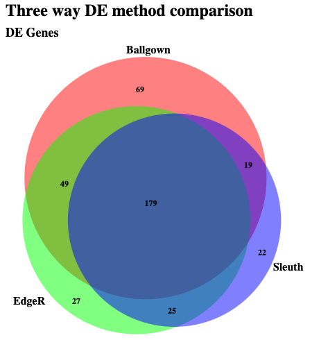
Take a look at the list of genes found to be significant according to all three methods: HISAT/StringTie/Ballgown, HISAT/HTseq-count/EdgeR, and Kallisto/Sleuth. Note here that for EdgeR the analysis was only done at the Gene level. So we will compare the gene lists. In the case of Kallisto we will determine genes where at least one transcript was significantly DE. Which is not quite the same thing as what is happening with the other two methods.
First produce a simple gene list from the sleuth significant transcripts file
cd $RNA_HOME/de
cat sleuth/results/UHR_vs_HBR_transcript_results_sig.tsv | cut -f 13 | sort | grep -v gene_name | uniq > sleuth_genes_with_de_transcripts.txt
wc -l *.txt
Once again we could visualize the overlap with a venn diagram. This can be done with simple web tools like:
cat ballgown_DE_gene_symbols.txt
cat DESeq2_DE_gene_symbols.txt
cat sleuth_genes_with_de_transcripts.txt
Alternatively you could view both lists in a web browser as you have done with other files. These three files should be here:
https://YOUR_PUBLIC_IPv4_ADDRESS/rnaseq/de/ballgown_DE_gene_symbols.txt https://YOUR_PUBLIC_IPv4_ADDRESS/rnaseq/de/DESeq2_DE_gene_symbols.txt https://YOUR_PUBLIC_IPv4_ADDRESS/rnaseq/de/sleuth_genes_with_de_transcripts.txt
If this works you should see an overlap that looks something like this:
Obtain an entire lane of RNA-seq data for a breast cancer cell line and matched ‘normal’ cell line here:
NOTE: do not attempt this unless you have a lot of free space on your machine (at least 250 GB)
Tumor (download)
Normal (download)
For more information on this data refer to this page: https://github.com/genome/gms/wiki/HCC1395-WGS-Exome-RNA-Seq-Data
Download the data
cd $RNA_HOME/data/
mkdir hcc1395
cd hcc1395
wget https://xfer.genome.wustl.edu/gxfer1/project/gms/testdata/bams/hcc1395/gerald_C1TD1ACXX_8_ACAGTG.bam
wget https://xfer.genome.wustl.edu/gxfer1/project/gms/testdata/bams/hcc1395/gerald_C2DBEACXX_3.bam
Convert BAM to FASTQ
Since the paths above will download BAM files but Kallisto expects FASTQ files for the read data. You will need to convert from BAM back to FASTQ. Try using Picard to do this.
Example BAM to FASTQ conversion commands (note that you need to specify the correct path for your Picard installation), followed by compressing the resulting FastQ files to save space:
java -Xmx2g -jar $PICARD SamToFastq INPUT=gerald_C1TD1ACXX_8_ACAGTG.bam FASTQ=hcc1395_tumor_R1.fastq SECOND_END_FASTQ=hcc1395_tumor_R2.fastq VALIDATION_STRINGENCY=LENIENT
gzip hcc1395_tumor*.fastq
java -Xmx2g -jar $PICARD SamToFastq INPUT=gerald_C2DBEACXX_3.bam FASTQ=hcc1395_normal_R1.fastq SECOND_END_FASTQ=hcc1395_normal_R2.fastq VALIDATION_STRINGENCY=LENIENT
gzip hcc1395_normal*.fastq
Download full transcriptome reference
You will have to get all transcripts instead of just those for a single chromosome. You will also have to create a new index for this new set of transcript sequences.
wget ftp://ftp.ensembl.org/pub/release-89/fasta/homo_sapiens/cdna/Homo_sapiens.GRCh38.cdna.all.fa.gz
Now repeat the concepts above to obtain abundance estimates for all genes.
kallisto index --index=Homo_sapiens.GRCh38.cdna.all_index Homo_sapiens.GRCh38.cdna.all.fa.gz

kallisto quant --index=Homo_sapiens.GRCh38.cdna.all_index --output-dir=normal --threads=4 --plaintext hcc1395/hcc1395_normal_R1.fastq.gz hcc1395/hcc1395_normal_R2.fastq.gz
kallisto quant --index=Homo_sapiens.GRCh38.cdna.all_index --output-dir=tumor --threads=4 --plaintext hcc1395/hcc1395_tumor_R1.fastq.gz hcc1395/hcc1395_tumor_R2.fastq.gz
Note:
time command in Unix to track how long the kallisto index and kallisto quant commands take.