Batch Correction Analysis

In this section we will use the ComBat-Seq tool in R (Bioconductor) to demonstrate the principles and application of batch correction. Due to the way our test data was generated (at a single center, at one time, with consistent methodology) we do NOT expect batch effects in these data. Therefore we will use a different (but highly related) dataset to demonstrate the impact of Batch correction in this module.
Introduction to batch correction
We highly recommend reading the entire ComBat-Seq manuscript by Yuqing Zhang, Giovanni Parmigiani, and W Evan Johnson. This manuscript does a beautiful job of briefly introducing the concept of batch correction and the differences between normalization and batch correction. If you find this exercise helpful in your research, please cite the ComBat-Seq paper (PMID: 33015620).
In particular, this excerpt covers the basics:
Genomic data are often produced in batches due to logistical or practical restrictions, but technical variation and differences across batches, often called batch effects, can cause significant heterogeneity across batches of data. Batch effects often result in discrepancies in the statistical distributions across data from different technical processing batches, and can have unfavorable impact on downstream biological analysis … Batch effects often cannot be fully addressed by normalization methods and procedures. The differences in the overall expression distribution of each sample across batch may be corrected by normalization methods, such as transforming the raw counts to (logarithms of) CPM, TPM or RPKM/FPKM, the trimmed mean of M values (TMM), or relative log expression (RLE). However, batch effects in composition, i.e. the level of expression of genes scaled by the total expression (coverage) in each sample, cannot be fully corrected with normalization. … While the overall distribution of samples may be normalized to the same level across batches, individual genes may still be affected by batch-level bias.
Introduction to this demonstration of a batch correction approach
For this exercise we have obtained public RNA-seq data from an extensive multi-platform comparison of sequencing platforms that also examined the impact of: (1) generating data at multiple sites, (2) using polyA vs ribo-reduction for enrichment, and (3) different levels of RNA degradation (PMID: 25150835): “Multi-platform and cross-methodological reproducibility of transcriptome profiling by RNA-seq in the ABRF Next-Generation Sequencing Study”.
This publication used the same UHR (cancer cell lines) and HBR (brain tissue) samples we have been using throughout this course. To examine a strong batch effect, we will consider a DE analysis of UHR vs HBR where we compare Ribo-depleted (“Ribo”) and polyA-enriched (“Poly”) samples.
Questions If we do DE analysis of UHR vs. HBR for replicates that are consistent with respect to Ribo-depletion or PolyA-enrichment, how does the result compare to when we mix the Ribo-depleted data and PolyA-enriched data together?
If you do batch correction and redo these comparisons does it make the results more comparable? i.e. can we correct for the technical differences introduced by the library construction approach and see the same biological differences? Can we improve our statistical power by then benefitting from more samples?
This is a bit contrived because there really are true biological differences expected for polyA vs. Ribo-depleted data. To counter this, we will limit the analysis to only know protein coding genes. For those genes we expect essentially the same biological answer when comparing UHR vs HBR expression patterns.
This exercise is also a bit simplistic in the sense that we have perfectly balanced conditions and batches. Our conditions of interest are: HBR (brain) vs. UHR (cancer cell line) expression patterns. Our batches are the two methods of processing: Riboreduction and PolyA enrichment. And we have 4 replicates of both conditions in both batches. To perform this kind of batch correction you need at least some representation of each of your conditions of interest in each batch. So, for example, if we processed all the HBR samples with Riboreduction and all the UHR samples with PolyA enrichment, we would be unable to model the batch effect vs the condition effect.
There are also other experiments from this published dataset we could use instead. For example, different levels of degradation?, data generated by different labs? Figure 1 and Figure 2 give a nice high level summary of all the data generated. We chose the Ribo-reduction and PolyA enrichment data for this exercise because we expect this would introduce a very strong batch effect. It is also the kind of thing that one could imagine really coming up in a meta-analysis where one you are pooling data from multiple studies. For example, imagine we find three published studies from three labs that all assayed some number of normal breast tissue and breast tumor. Each used a different approach to generate their data but they all involved this same biological comparison and by combining the three datasets we hope to substantially increase our power. If we can correct for batch effects arising from the three labs, this may be successful.
Samples abbreviations used in the following analysis
- HBR -> Human Brain Reference, Biological condition (pool of adult brain tissues)
- UHR -> Universal Human Reference, Biological condition (pool of cancer cell lines)
- Ribo -> Library preparation method using ribosomal reduction, Batch group
- Poly -> Library preparation method using polyA enrichment, Batch group
- 1-4 -> Replicate number: 1, 2, 3, 4.
Perform principal component analysis (PCA) on the uncorrected counts
PCA analysis can be used to identify potential batch effects in your data. The general strategy is to use PCA to identify patterns of similarity/difference in the expression signatures of your samples and to ask whether it appears to be driven by the expected biological conditions of interest. The PCA plot can be labeled with the biological conditions and also with potential sources of batch effects such as: sequencing source, date of data generation, lab technician, library construction kit batches, matrigel batches, mouse litters, software or instrumentation versions, etc.
Principal component analysis is a dimensionality-reduction method that can be applied to large datasets (e.g. thousands of gene expression values for many samples). PCA tries to represent a large set of variables as a smaller set of variables that maximally capture the information content of the larger set. PCA is a general exploratory data analysis approach with many applications and nuances, the details of which are beyond the scope of this demonstration of batch effect correction. However, in the context of this module, PCA provides a way to visualize samples as “clusters” based on their overall pattern of gene expression values. The composition and arrangement of these clusters (usually visualized in 2D or interactive 3D plots) can be helpful in interpreting high level differences between samples and testing prior expectations about the similarity between conditions, replicates, etc.
We will perform PCA analysis before AND after batch correction. Samples will be labelled according to biological condition (UHR vs HBR) and library preparation type (Ribo vs PolyA).
Does the analysis below suggest that sample grouping according to PCA is being influenced by batch?
Perform the following analyses in R:
#Define working dir paths
# datadir = "/cloud/project/data/bulk_rna"
# outdir = "/cloud/project/outdir"

datadir = "~/workspace/rnaseq/batch_correction"
outdir = "~/workspace/rnaseq/batch_correction/outputs"

if (!dir.exists(outdir)) dir.create(outdir)


#load neccessary libraries
library("sva") #Note this exercise requires sva (>= v3.36.0) which is only available for R (>= v4.x)
library("ggplot2")
library("gridExtra")
library("edgeR")
library("UpSetR")
library(grid)

#load in the uncorrected data as raw counts
setwd(datadir)
uncorrected_data = read.table("GSE48035_ILMN.Counts.SampleSubset.ProteinCodingGenes.tsv", header = TRUE, sep = "\t", as.is = c(1,2))
setwd(outdir)

#simplify the names of the data columns
# (A = Universal Human Reference RNA and B = Human Brain Reference RNA)
# RNA = polyA enrichment and RIBO = ribosomal RNA depletion
# 1, 2, 3, 4 are replicates
names(uncorrected_data) = c("Gene", "Chr", "UHR_Ribo_1", "UHR_Ribo_2", "UHR_Ribo_3", "UHR_Ribo_4", "HBR_Ribo_1", "HBR_Ribo_2", "HBR_Ribo_3", "HBR_Ribo_4",
                            "UHR_Poly_1", "UHR_Poly_2", "UHR_Poly_3", "UHR_Poly_4", "HBR_Poly_1", "HBR_Poly_2", "HBR_Poly_3", "HBR_Poly_4")
sample_names = names(uncorrected_data)[3:length(names(uncorrected_data))]

#review data structure
head(uncorrected_data)
dim(uncorrected_data)

#define conditions, library methods, and replicates
conditions = c("UHR", "UHR", "UHR", "UHR", "HBR", "HBR", "HBR", "HBR", "UHR", "UHR", "UHR", "UHR", "HBR", "HBR", "HBR", "HBR")
library_methods = c("Ribo", "Ribo", "Ribo", "Ribo", "Ribo", "Ribo", "Ribo", "Ribo", "Poly", "Poly", "Poly", "Poly", "Poly", "Poly", "Poly", "Poly")
replicates = c(1, 2, 3, 4, 1, 2, 3, 4, 1, 2, 3, 4, 1, 2, 3, 4)

#calculate principal components for the uncorrected data
pca_uncorrected_obj = prcomp(uncorrected_data[,sample_names])

#pull PCA values out of the PCA object
pca_uncorrected = as.data.frame(pca_uncorrected_obj[2]$rotation)

#determine the percentage of variance explained by each PC
variance = (pca_uncorrected_obj$sdev)^2
percent_variance = (variance / sum(variance)) * 100

#assign labels to the data frame
pca_uncorrected[,"condition"] = conditions
pca_uncorrected[,"library_method"] = library_methods
pca_uncorrected[,"replicate"] = replicates

#plot the PCA
#create a classic 2-dimension PCA plot (first two principal components) with conditions and library methods indicated
pc1_label = paste("PC1 (", round(percent_variance[1], digits=1), "% variance explained)", sep="")
pc2_label = paste("PC2 (", round(percent_variance[2], digits=1), "% variance explained)", sep="")

cols <- c("UHR" = "#481567FF", "HBR" = "#1F968BFF")
p1 = ggplot(data = pca_uncorrected, aes(x = PC1, y = PC2, color = condition, shape = library_method))
p1 = p1 + geom_point(size = 3)
p1 = p1 + stat_ellipse(type = "norm", linetype = 2)
p1 = p1 + labs(title = "PCA, RNA-seq counts for 16 HBR/UHR and Ribo/PolyA samples (uncorrected data)", color = "Condition", shape="Library Method")
p1 = p1 + labs(x = pc1_label, y = pc2_label)
p1 = p1 + scale_colour_manual(values = cols)
Introduction to Bioconductor SVA and ComBat-Seq in R
The ComBat-Seq package is made available as part of the SVA package for Surrogate Variable Analysis. This package is a collection of methods for removing batch effects and other unwanted variation in large datasets. It includes the ComBat method that has been widely used for batch correction of gene expression datasets, especially those generated on microarray platforms. ComBat-Seq is a modification of the ComBat approach. ComBat-Seq has been tailored to the count based data of bulk RNA-seq datasets. Particular advantages of the ComBat-Seq approach are that it: (1) uses a negative binomial regression model (the negative binomial distribution is thought to model the characteristics of bulk RNA-seq count data), and (2) allows the output of corrected data that retain the count nature of the data and can be safely fed into many existing methods for DE analysis (such as EdgeR and DESeq2).
ComBat-Seq has a relatively short list of arguments, and for several of these we will use the default setting. Very basic documentation of these arguments can be found here and here.
Our attempt to explain each of the ComBat-Seq arguments (for optional arguments, default is shown):
counts. This is your matrix of gene expression read counts (raw counts). Each row is a gene, each column is a sample, and each cell has an integer count for the number of RNA-seq counts observed for that gene/sample combination. In R we want this data to be passed into ComBat-Seq in matrix format (useas.matrix()if neccessary).batch. This is a vector describing the batches you are concerned about. For example, if you have eight samples that you created RNA-seq data for, but for the first four you used library kit (A) and for the last four samples you used library kit (B). In this situation you would define yourbatchvector as:c(1,1,1,1,2,2,2,2).group = NULL. This is a vector describing your biological condition of interest. For example, if your experiment involved pairs of drug treated and untreated cells, and you did 4 biological replicates. You would define yourgroupvector as: c(1,2,1,2,1,2,1,2).covar_mod = NULL. If you have multiple biological conditions of interest, you can define these withcovar_mod(covariates) instead ofgroup. For example, lets assume we have the same experiment as described above, except that we did four replicates (treated vs untreated pairs), but we alternated use of male and female cells for each of the replicates. You then would define a covariate matrix to supply tocovar_modas follows:
  #treatment_group = c(1,2,1,2,1,2,1,2)
  #sex_group = c(1,1,2,2,1,1,2,2)
  #covariate_matrix = cbind(treatment_group, sex_group)
full_mod = TRUE. If TRUE include the condition of interest in model. Generally we believe this should be set to the default TRUE. We have yet to find a cohesive explanation for a situation where one would want this to be FALSE.shrink = FALSE. Whether to apply shrinkage on parameter estimation.shrink.disp = FALSE. Whether to apply shrinkage on dispersion.gene.subset.n = NULL. Number of genes to use in empirical Bayes estimation, only useful when shrink = TRUE.
A detailed discussion of shrinkage (related to the shrink, shrink.disp, and gene_subset.n arguments is beyond the scope of this tutorial. Briefly, shrinkage refers to a set of methods that attempt to correct for gene-specific variability in the counts observed in RNA-seq datasets. More specifically, it relates to the dispersion parameter of the negative binomial distribution used to model RNA-seq count data that can suffer from overdispersion. The dispersion parameter describes how much variance deviates from the mean. In simple terms, shrinkage methods are an attempt to correct for problematic dispersion. A more detailed discussion of these statistical concepts can be found in the DESeq2 paper. However, for our purposes here, the bottom line is that the ComBat-Seq authors state that “We have shown that applying empirical Bayes shrinkage is not necessary for ComBat-seq because the approach is already sufficiently robust due to the distributional assumption.” So we will leave these arguments at their default FALSE settings.
Demonstration of ComBat-Seq on the UHR/HBR data with two library types (Ribo/Poly)
Continuing the R session started above, use ComBat-Seq to perform batch correction as follows:
#perform the batch correction

#first we need to transform the format of our groups and batches from names (e.g. "UHR", "HBR", etc.) to numbers (e.g. 1, 2, etc.)
#in the command below "sapply" is used to apply the "switch" command to each element and convert names to numbers as we define
groups = sapply(as.character(conditions), switch, "UHR" = 1, "HBR" = 2, USE.NAMES = FALSE)
batches = sapply(as.character(library_methods), switch, "Ribo" = 1, "Poly" = 2, USE.NAMES = FALSE)

#now run ComBat_seq
corrected_data = ComBat_seq(counts = as.matrix(uncorrected_data[,sample_names]), batch = batches, group = groups)

#join the gene and chromosome names onto the now corrected counts from ComBat_seq
corrected_data = cbind(uncorrected_data[, c("Gene", "Chr")], corrected_data)

#compare dimensions of corrected and uncorrected data sets
dim(uncorrected_data)
dim(corrected_data)

#visually compare values of corrected and uncorrected data sets
head(uncorrected_data)
head(corrected_data)
Perform PCA analysis on the batch corrected data and contrast with the uncorrected data
As performed above, use PCA to examine whether batch correction changes the grouping of samples by the expression patterns. Does the corrected data cluster according to biological condition (UHR vs HBR) better now regardless of library preparation type (Ribo vs PolyA)?
#calculate principal components for the uncorrected data
pca_corrected_obj = prcomp(corrected_data[, sample_names])

#pull PCA values out of the PCA object
pca_corrected = as.data.frame(pca_corrected_obj[2]$rotation)

#determine the percentage of variance explained by each PC
variance = (pca_corrected_obj$sdev)^2
percent_variance = (variance / sum(variance)) * 100

#assign labels to the data frame
pca_corrected[,"condition"] = conditions
pca_corrected[,"library_method"] = library_methods
pca_corrected[,"replicate"] = replicates

#as above, create a PCA plot for comparison to the uncorrected data
pc1_label = paste("PC1 (", round(percent_variance[1], digits=1), "% variance explained)", sep="")
pc2_label = paste("PC2 (", round(percent_variance[2], digits=1), "% variance explained)", sep="")
cols <- c("UHR" = "#481567FF", "HBR" = "#1F968BFF")

p2 = ggplot(data = pca_corrected, aes(x = PC1, y = PC2, color = condition, shape = library_method))
p2 = p2 + geom_point(size = 3)
p2 = p2 + stat_ellipse(type = "norm", linetype = 2)
p2 = p2 + labs(title = "PCA, RNA-seq counts for 16 HBR/UHR and Ribo/PolyA samples (batch corrected data)", color = "Condition", shape = "Library Method")
p2 = p2 + labs(x = pc1_label, y = pc2_label)
p2 = p2 + scale_colour_manual(values = cols)

pdf(file = "Uncorrected-vs-BatchCorrected-PCA.pdf")
grid.arrange(p1, p2, nrow = 2)
dev.off()
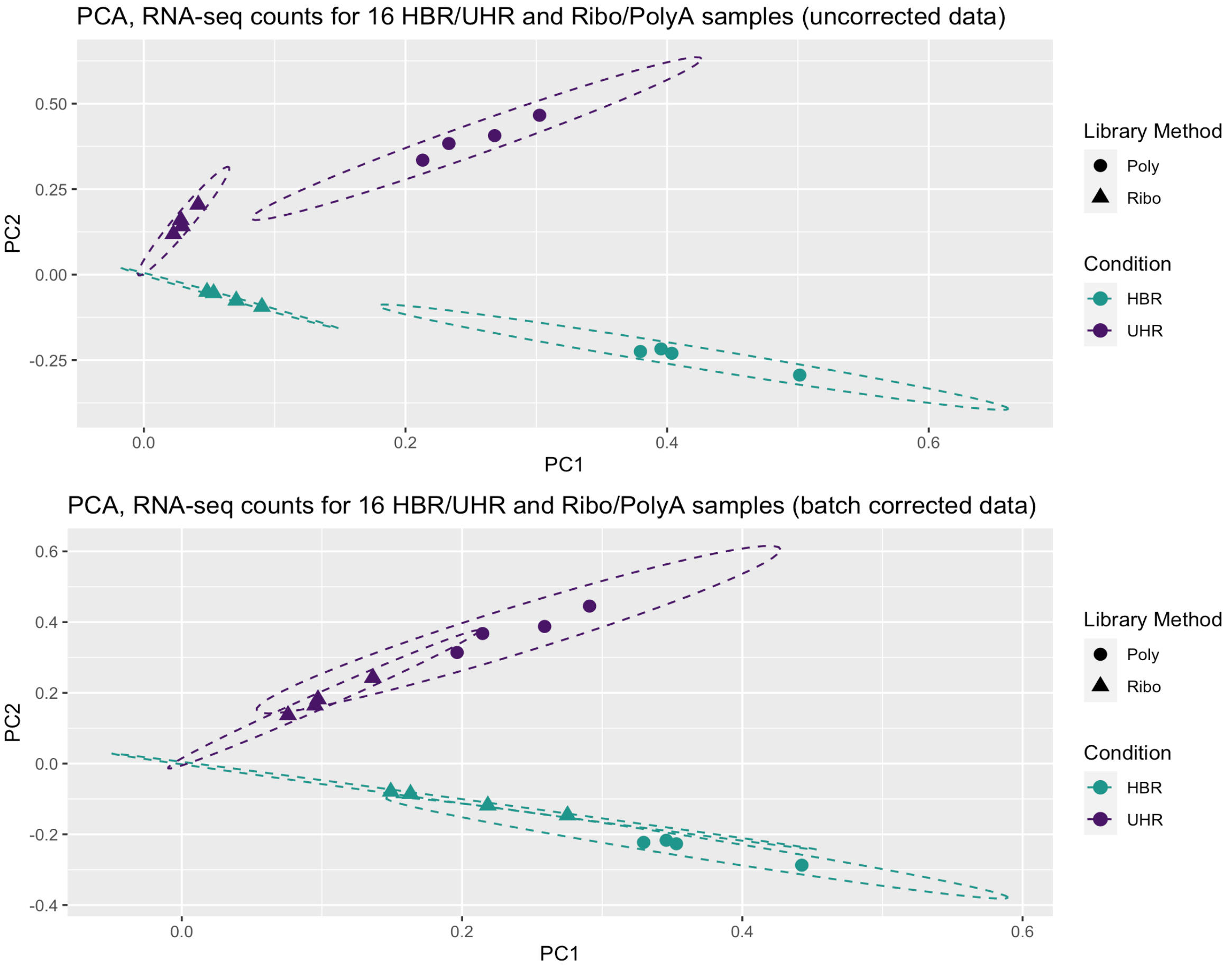
If the above analysis worked you should have an image that looks like this:

Note that prior to correction the UHR samples are separate from the HBR samples. Note that the PolyA and Ribo-reduction samples are also separated. The 16 samples group into 4 fairly distinct clusters. In other words, the overall expression signatures of these samples seem to reflect both the biological condition (UHR vs HBR) and library construction approach (Ribo vs PolyA).
However, after correcting for the batch effect of library construction approach, we see a marked improvement. The library construction approach still seems to be noticeable, but the 16 samples now essentially group into two distinct clusters: HBR and UHR.
Perform differential expression analysis of the corrected and uncorrected data
How does batch correction influence differential gene expression results? Use UpSet plots to examine the overlap of significant DE genes found for the following comparisons:
- UHR-Ribo vs HBR-Ribo (same library type, 4 vs 4 replicates)
- UHR-Poly vs HBR-Poly (same library type, 4 vs 4 replicates)
- UHR-Ribo vs HBR-Poly (different library types, 4 vs 4 replicates)
- UHR-Poly vs HBR-Ribo (different library types, 4 vs 4 replicates)
- UHR-Comb vs HBR-Comb (combined library types, 8 vs 8 replicates)
These five differential expression analysis comparisons will be performed with both the uncorrected and corrected data.
- Does correction increase agreement between the five comparisons?
- Does it appear to increase statistical power when combining all 8 replicates of UHR and HBR?
- What do we expect to see for comparisons like UHR-Ribo vs HBR-Poly before and after batch correction? Do we expect correction to increase or decrease the number of significant results?
Explore these questions by continuing on with the R session started above and doing the following:
#perform differential expression analysis on the uncorrected data and batch corrected data sets

#first define the sets of samples to be compared to each other
uhr_ribo_samples = c("UHR_Ribo_1", "UHR_Ribo_2", "UHR_Ribo_3", "UHR_Ribo_4")
uhr_poly_samples = c("UHR_Poly_1", "UHR_Poly_2", "UHR_Poly_3", "UHR_Poly_4")
hbr_ribo_samples = c("HBR_Ribo_1", "HBR_Ribo_2", "HBR_Ribo_3", "HBR_Ribo_4")
hbr_poly_samples = c("HBR_Poly_1", "HBR_Poly_2", "HBR_Poly_3", "HBR_Poly_4")
uhr_samples = c(uhr_ribo_samples, uhr_poly_samples)
hbr_samples = c(hbr_ribo_samples, hbr_poly_samples)

#create a function that will run edgeR (DE analysis) for a particular pair of sample sets
run_edgeR = function(data, group_a_name, group_a_samples, group_b_samples, group_b_name){
  #create a list of all samples for this current comparison
  samples_for_comparison = c(group_a_samples, group_b_samples)

  #define the class factor for this pair of sample sets
  class = factor(c(rep(group_a_name, length(group_a_samples)), rep(group_b_name, length(group_b_samples))))

  #create a simplified data matrix for only these samples
  rawdata = data[, samples_for_comparison]

  #store gene names for later
  genes = rownames(data)
  gene_names = data[,"Gene"]

  #make DGElist object
  y = DGEList(counts = rawdata, genes = genes, group = class)

  #perform TMM normalization
  y = calcNormFactors(y)

  #estimate dispersion
  y = estimateCommonDisp(y, verbose = TRUE)
  y = estimateTagwiseDisp(y)

  #perform the differential expression test
  et = exactTest(y)

  #print number of up/down significant genes at FDR = 0.05 significance level and store the DE status in a new variable (de)
  de = decideTests(et, adjust.method = "fdr", p = 0.05)
  summary(de)

  #create a matrix of the DE results
  mat = cbind(
    genes,
    gene_names,
    sprintf("%0.3f", log10(et$table$PValue)),
    sprintf("%0.3f", et$table$logFC)
  )

  #create a version of this matrix that is limited to only the *significant* results
  mat = mat[as.logical(de),]

  #add name to the columns of the final matrix
  colnames(mat) <- c("Gene", "Gene_Name", "Log10_Pvalue", "Log_fold_change")

  return(mat)
}

#run the five comparisons through edgeR using the *uncorrected data*
uhr_ribo_vs_hbr_ribo_uncorrected = run_edgeR(data = uncorrected_data, group_a_name = "UHR", group_a_samples = uhr_ribo_samples, group_b_name = "HBR", group_b_samples = hbr_ribo_samples)
uhr_poly_vs_hbr_poly_uncorrected = run_edgeR(data = uncorrected_data, group_a_name = "UHR", group_a_samples = uhr_poly_samples, group_b_name = "HBR", group_b_samples = hbr_poly_samples)
uhr_ribo_vs_hbr_poly_uncorrected = run_edgeR(data = uncorrected_data, group_a_name = "UHR", group_a_samples = uhr_ribo_samples, group_b_name = "HBR", group_b_samples = hbr_poly_samples)
uhr_poly_vs_hbr_ribo_uncorrected = run_edgeR(data = uncorrected_data, group_a_name = "UHR", group_a_samples = uhr_poly_samples, group_b_name = "HBR", group_b_samples = hbr_ribo_samples)
uhr_vs_hbr_uncorrected = run_edgeR(data = uncorrected_data, group_a_name = "UHR", group_a_samples = uhr_samples, group_b_name = "HBR", group_b_samples = hbr_samples)

#run the same five comparisons through edgeR using the *batch corrected data*
uhr_ribo_vs_hbr_ribo_corrected = run_edgeR(data = corrected_data, group_a_name = "UHR", group_a_samples = uhr_ribo_samples, group_b_name = "HBR", group_b_samples = hbr_ribo_samples)
uhr_poly_vs_hbr_poly_corrected = run_edgeR(data = corrected_data, group_a_name = "UHR", group_a_samples = uhr_poly_samples, group_b_name = "HBR", group_b_samples = hbr_poly_samples)
uhr_ribo_vs_hbr_poly_corrected = run_edgeR(data = corrected_data, group_a_name = "UHR", group_a_samples = uhr_ribo_samples, group_b_name = "HBR", group_b_samples = hbr_poly_samples)
uhr_poly_vs_hbr_ribo_corrected = run_edgeR(data = corrected_data, group_a_name = "UHR", group_a_samples = uhr_poly_samples, group_b_name = "HBR", group_b_samples = hbr_ribo_samples)
uhr_vs_hbr_corrected = run_edgeR(data = corrected_data, group_a_name = "UHR", group_a_samples = uhr_samples, group_b_name = "HBR", group_b_samples = hbr_samples)

#how much of a difference does batch correction make when doing the comparison of all UHR vs all HBR samples?
dim(uhr_vs_hbr_uncorrected)
dim(uhr_vs_hbr_corrected)

#create upset plots to summarize the overlap between the comparisons performed above

#first create upset plot from the *uncorrected* data
listInput1 = list("4 UHR Ribo vs 4 HBR Ribo" = uhr_ribo_vs_hbr_ribo_uncorrected[, "Gene"],
                  "4 UHR Poly vs 4HBR Poly" = uhr_poly_vs_hbr_poly_uncorrected[, "Gene"],
                  "4 UHR Ribo vs 4 HBR Poly" = uhr_ribo_vs_hbr_poly_uncorrected[, "Gene"],
                  "4 UHR Poly vs 4 HBR Ribo" = uhr_poly_vs_hbr_ribo_uncorrected[, "Gene"],
                  "8 UHR vs 8 HBR" = uhr_vs_hbr_uncorrected[, "Gene"])

pdf(file = "Uncorrected-UpSet.pdf", onefile = FALSE)
upset(fromList(listInput1), order.by = "freq", number.angles = 45, point.size = 3)
dev.off()

#now create an upset plot from the *batch corrected* data
listInput2 = list("4 UHR Ribo vs 4 HBR Ribo" = uhr_ribo_vs_hbr_ribo_corrected[,"Gene"],
                  "4 UHR Poly vs 4 HBR Poly" = uhr_poly_vs_hbr_poly_corrected[,"Gene"],
                  "4 UHR Ribo vs 4 HBR Poly" = uhr_ribo_vs_hbr_poly_corrected[,"Gene"],
                  "4 UHR Poly vs 4 HBR Ribo" = uhr_poly_vs_hbr_ribo_corrected[,"Gene"],
                  "8 UHR vs 8 HBR" = uhr_vs_hbr_corrected[,"Gene"])

pdf(file = "BatchCorrected-UpSet.pdf", onefile = FALSE)
upset(fromList(listInput2), order.by = "freq", number.angles=45, point.size=3)
dev.off()

#write out the final set of DE genes where all UHR and HBR samples were compared using the corrected data
write.table(uhr_vs_hbr_corrected, file = "DE_genes_uhr_vs_hbr_corrected.tsv", quote = FALSE, row.names = FALSE, sep = "\t")

#To exit R type the following
#quit(save = "no")
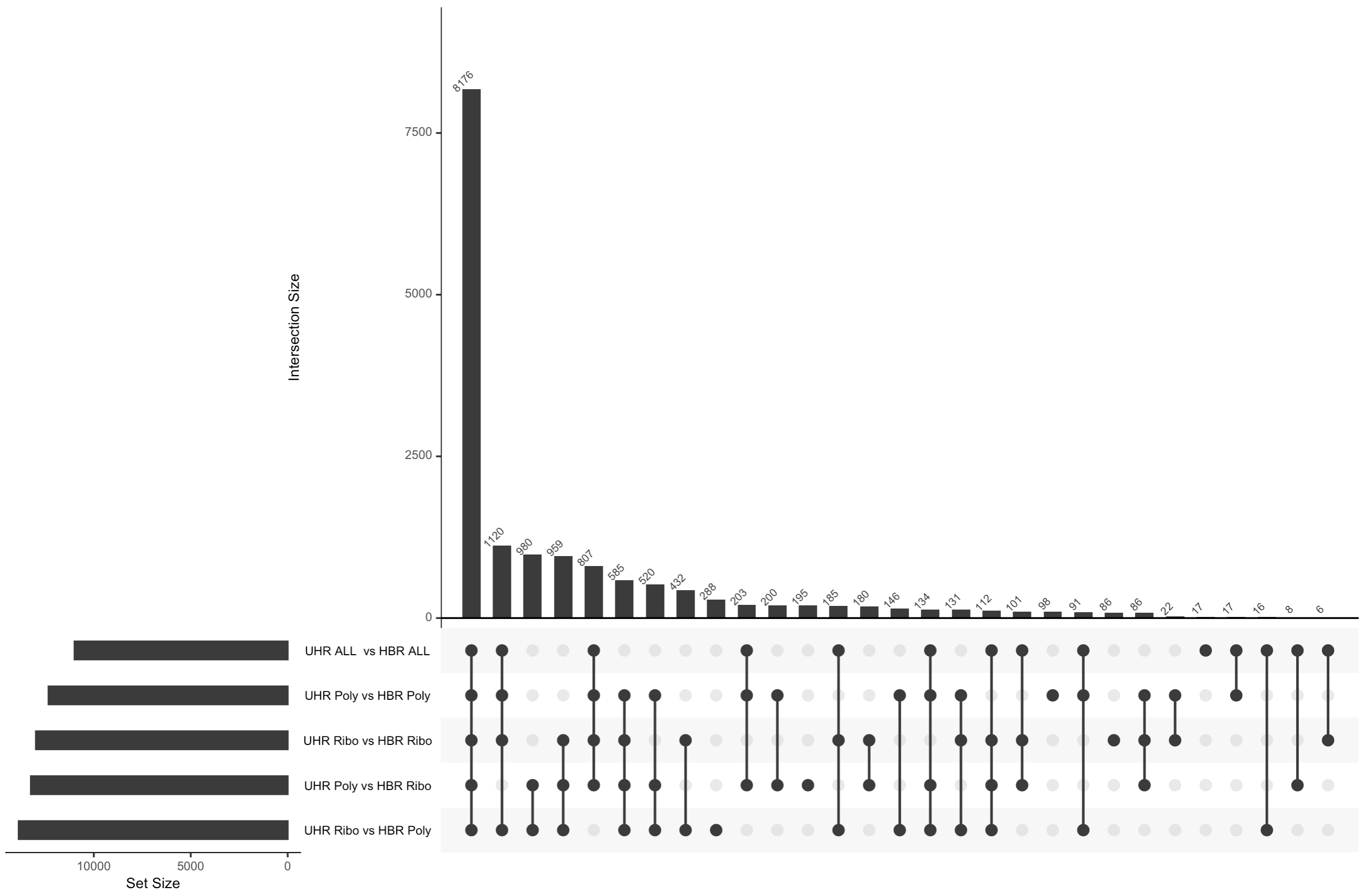
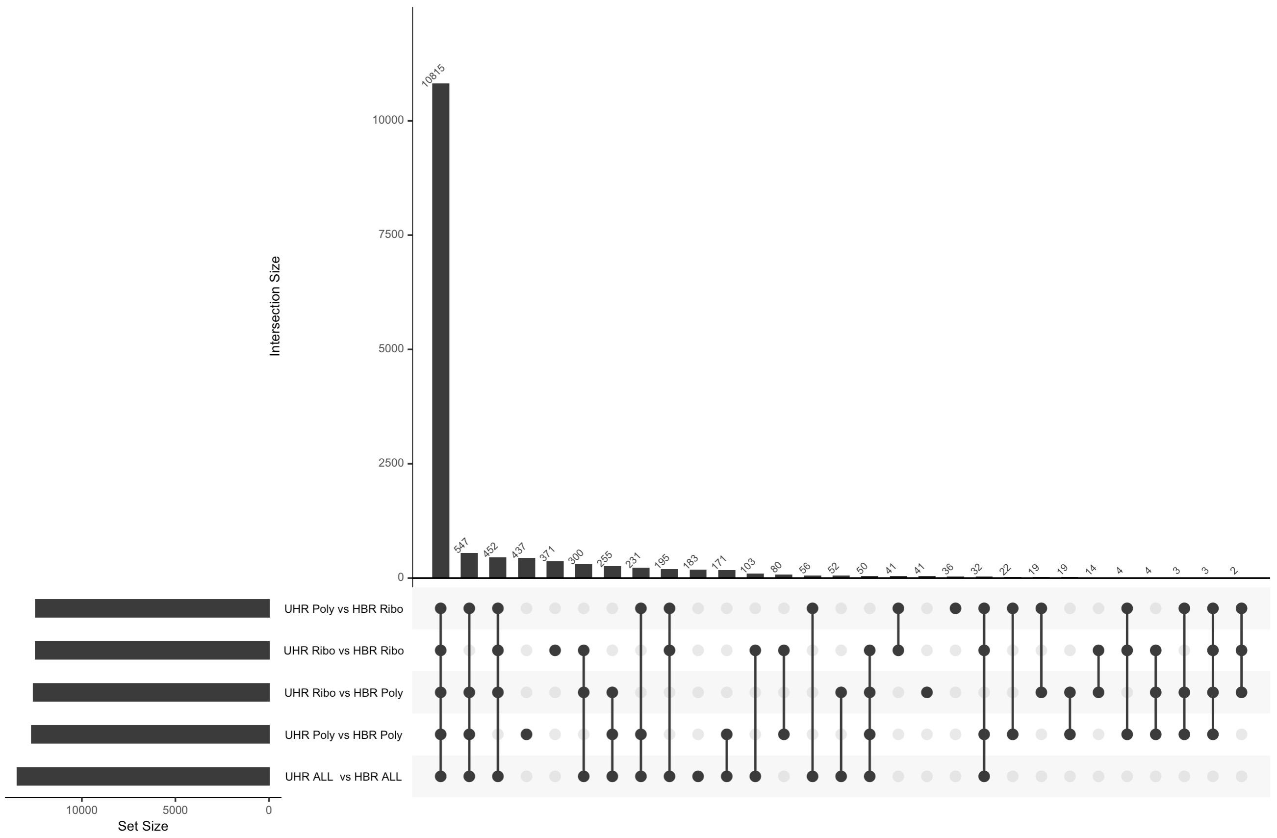
Note that an UpSet plot is an alternative to a Venn Diagram. It shows the overlap (intersection) between an arbitrary number of sets of values. In this case we are comparing the list of genes identified as significantly DE by five different comparisons. The black circles connected by a line indicate each combination of sets being considered. The bar graph above each column shows how many genes are shared across those sets. For example, the first column has all five black circles. The bar above that column indicates how many genes were found in all five DE comparisons performed.
What differs in each comparison is:
- whether we are comparing replicates prepared with the same library construction approach (Ribo reduction or PolyA) or whether we are comparing data prepared with different approaches
- whether we are comparing 4 UHR vs 4 HBR replicates according to these library construction approaches, or pooling all 8 UHR and all 8 HBR samples (ignoring their different library types)
- whether we are doing these comparisons before or after batch correction
Before batch correction

After batch correction

There are several notable observations from the analysis above and the two UpSet plots.
- In the uncorrected data, we actually see more DE genes when comparing a mix of library contruction approaches (e.g. UHR-Ribo vs UHR-Poly). There are likely false positives in these results. i.e. Genes that appear to be different between UHR and HBR, but where the difference is actually caused by differences in the library preparation not the biology.
- If we combine all 8 samples together for each biological condition we can see that we actually get considerably fewer significant genes with the uncorrected data. Presumably this is because we are now introducing noise caused by a mix of different library construction approaches and this impacts the statistical analysis (more variability).
- When we apply batch correction, we see that now all five comparisons tend to agree with each other for the most part on what genes are differentially expressed. Overall agreement across comparisons is improved.
- With the batch corrected data we now see that combining all 8 samples actually improves statistical power and results in a larger number of significant DE genes relative to the 4 vs 4 comparisons. This is presumably the most accurate result of all the comparisons we did.
