Posts
My thoughts and ideas
Welcome to the blog
My thoughts and ideas
Introduction to bioinformatics for RNA sequence analysis
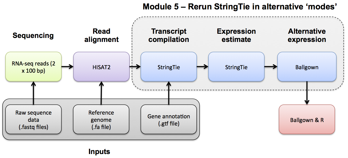
Use Stringtie to merge predicted transcripts from all libraries into a unified transcriptome. Refer to the Stringtie manual for a more detailed explanation:
https://ccb.jhu.edu/software/stringtie/index.shtml?t=manual
Options specified below:
assembly_GTF_list.txt is a text file “manifest” with a list (one per line) of GTF files that you would like to merge together into a single GTF file.–rf tells StringTie that our data is stranded and to use the correct strand specific mode (i.e. assume a stranded library fr-firststrand).-p 4 tells stringtie to use eight CPUs-o tells stringtie to write output to a particular file or directory-G tells stringtie where to find reference gene annotations. It will use these annotations to gracefully merge novel isoforms (for de novo runs) and known isoforms and maximize overall assembly quality.Merge all 6 Stringtie results so that they will have the same set of transcripts for comparison purposes:
For reference guided mode:
cd $RNA_HOME/expression/stringtie/ref_guided/
ls -1 *Rep*/transcripts.gtf > assembly_GTF_list.txt
cat assembly_GTF_list.txt
stringtie --rf --merge -p 4 -o stringtie_merged.gtf -G $RNA_REF_GTF assembly_GTF_list.txt
What do the resulting transcripts look like?
awk '{if($3=="transcript") print}' stringtie_merged.gtf | cut -f 1,4,9 | less
Press q to exit the less viewer
Compare reference guided transcripts to the known annotations. This allows us to assess the quality of transcript predictions made from assembling the RNA-seq data. For more details, refer to the Stringtie GFF Utilities and Cuffcompare manuals.
gffcompare -r $RNA_REF_GTF -o gffcompare stringtie_merged.gtf
cat gffcompare.stats
What does the merged annotation look like after comparing it to known annotation? How are the GTF lines different?
awk '{if($3=="transcript") print}' gffcompare.annotated.gtf | cut -f 1,4,9 | less
Press ‘q’ to exit the less viewer
For de novo mode (again, we do not provide an Ensembl GTF):
cd $RNA_HOME/expression/stringtie/de_novo/
ls -1 *Rep*/transcripts.gtf > assembly_GTF_list.txt
cat assembly_GTF_list.txt
stringtie --rf --merge -p 4 -o stringtie_merged.gtf assembly_GTF_list.txt
Compare the de novo merged transcripts to the known annotations:
gffcompare -r $RNA_REF_GTF -o gffcompare stringtie_merged.gtf
cat gffcompare.stats