Cancer cell identification
Often when we’re analyzing cancer samples using scRNAseq, we need to identify tumor cells from healthy cells. Usually, we know what kind of celltype we expect the tumor cells to be (epithelial cells for bladder cancer, B cells for a B cell lymphoma, etc.), but we may want to distinguish tumor cells from normal cells of the same celltype for various reasons such as DE analyses. Also, since we are drawing conclusions related to gene expression from these comparisons, we may want to identify tumor cells using methods that are orthogonal to the genes expressed by the tumor cells. To that end, two common methods used are identifying either mutations or copy number alterations in scRNAseq data.
In the case of mutations, one will typically carry out mutation calling from DNA sequencing data (ideally from tumor-normal paired samples) and then ‘look’ for those mutations in the scRNAseq data’s BAM files using a tool like VarTrix. Because of the sparsity of single cell data, and its end bias (5’ or 3’ depending on the kit), it is unlikely that we can get every tumor cell from this approach, however it is likely that we can be pretty confident in the tumor cells we do identify.
For copy number alterations (CNAs), there are various tools that try to detect CNAs in tumor cells like CONICSmat and InferCNV. They rely on a similar principle of using the counts matrix to identify regions of the genome that collectively have higher or lower expression and that if (say) 100+ genes in the same region have higher (or lower) expression it is likely that that is due to a copy number gain (or loss) as opposed to their being upregulated (or downregulated).
Finding tumor cells based on Copy number data
If you are working in a tumor sample where you expect to find CNAs, looking for copy number alterations in the scRNAseq data can be one way to identify tumor cells. In our case, whole genome sequencing was done on the cell line used for the mouse models, so we have some confidently determined CNAs we expect to find in the scRNAseq data-
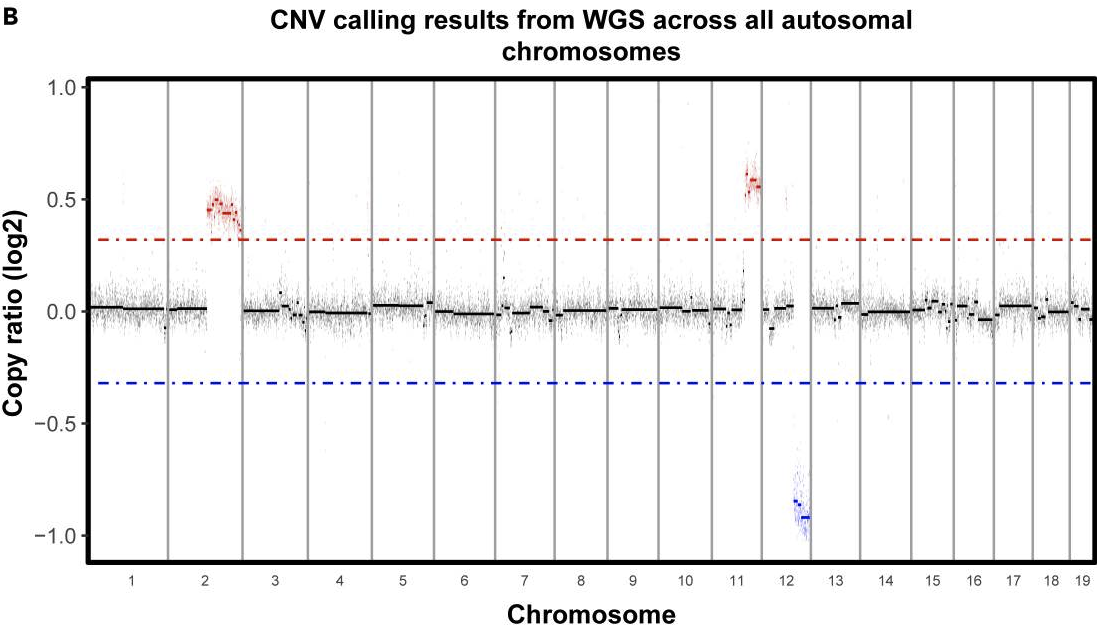
As we can see above, we expect to find gains in chromosome 2 and 11 and a loss in chromosome 12.
We will use CONICSmat to identify cells with CNAs in our scRNAseq data. While there is more information available on their GitHub tutorial and paper, briefly, CONICSmat fits a two-component Gaussian mixture model for each chromosomal region, and uses a Bayesian Information Criterion (BIC) statistical test to ask if a 1-component model (all cells are the same and there’s no CNA) fits better than a 2-component model (some cells have altered copy number compared to others). Here, a better fit is defined by a lower BIC score. Note that since we are only using the gene by cell counts matrix, average expression of genes in that chromosomal region is used as a proxy for a CNA. The key to most single-cell CNA based tools is that we need both tumor cells and non-tumor cells in our analysis as a copy number gain or loss in the tumor cells can only be measured relative to healthy cells. While CONICSmat can be run on all cells in the sample together, for our purposes, we will subset the object to Epithelial cells and B cells so that it can run more efficiently. CONICSmat is a somewhat computationally intensive tool, so we will start by clearing our workspace using the broom icon on the top right pane, and also click on the drop-down menu with a piechart beside it and select Free unused memory.
#make sure you have cleared your workspace and 'freed unused space' otherwise you may run into issues later on!

#start by loading in the libraries and the preprocessed Seurat object
library("Seurat")
library("ggplot2")
library("cowplot")
library("dplyr")
library("Matrix")
library("hdf5r")
library("CONICSmat")
library("showtext")

merged <- readRDS('outdir_single_cell_rna/preprocessed_object.rds')

#subset Seurat object to only include epithelial cells and B cells
merged <- SetIdent(merged, value = 'immgen_singler_main')
merged_subset <- subset(merged, idents=c('B cells', 'Epithelial cells'))

#as always double check that the number of cells match our expectations
table(merged$immgen_singler_main)
table(merged_subset$immgen_singler_main)
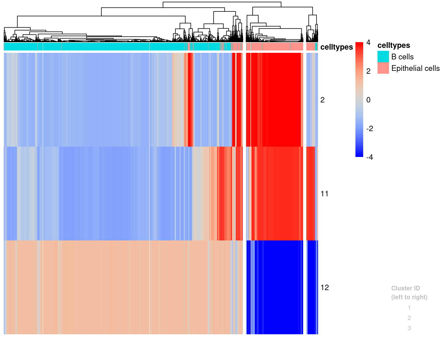
Now we can look into running CONICSmat! It is run in a few steps and requires us to look at some outputs along the way and define some thresholds. Tha main inputs CONICSmat needs are a Seurat counts matrix, a regions file specifying genomic regions, and a gene_pos file that has the genomic coordinates of all the genes. After we run the plotAll function, we will get a PDF file with results from the BIC test for every chromosomal region. We will look through this file to determine an appropriate BIC difference threshold that will help capture true CNA events. The BIC difference is (BIC 1 component score) - (BIC 2 component score), and a greater difference suggests a higher chance of a ‘real’ CNA event. Once we have a confident set of CNAs, we will use that information to cluster the cells in a heatmap wherein the heatmap is colored by z-scores calculated from the normalized average expression values.
#Normalize Seurat counts matrix using CONICsmat normMat function
conicsmat_expr <- CONICSmat::normMat(as.matrix(Seurat::GetAssayData(merged_subset, assay = 'RNA', layer = 'counts')))

#Get chromosomal positions of genes in the expression matrix
gene_pos=getGenePositions(rownames(conicsmat_expr), ensembl_version = "https://oct2022.archive.ensembl.org/", species = "mouse")

#Get coordinates for each region of interest (in our case we'll just use chromosome coordinates)
regions=read.table("/cloud/project/data/single_cell_rna/reference_files/chromosome_full_positions_mm10.txt",sep="\t",header = T, row.names = 1)


#Filter out uninformative genes aka genes that are expressed in less than 5 cells (that was the default given by CONICSmat)
conicsmat_expr=filterMatrix(conicsmat_expr,gene_pos[,"mgi_symbol"],minCells=5)

#Calculate normalization factor for each cell- this centers the gene expression in each cell around the mean.
#(Need this because the more genes that are expressed in a cell, the less reads are 'available' per gene)
normFactor=calcNormFactors(conicsmat_expr)

#Fit the 2 component Gaussian mixture model for each region to determine if the region has a CNA.
## This step outputs a PDF with a page for each region in the regions file that we can look through to determine which regions are likely to have a CNA.
## It also outputs a BIC_LR.txt file that summarizes the BIC scores and adj p-values for each region
l=plotAll(conicsmat_expr,normFactor,regions,gene_pos,"outdir_single_cell_rna/conic_plotall")
Let’s look through the conic_plotall_CNVs.pdf file. Looking through the results, we can see clear bimodal distributions for chromosomes 2, 11, and 12, and we see a corresponding lower BIC score for the 2 component model in these cases. However, we also see a low BIC score for cases like chromosome 5 even though we don’t see a bimodal distribution, and this may contribute to noisy results when we apply a BIC threshold. Looking at these barplots, a BIC threshold of around 800 might help filter out the noise, so let’s see the results with the default threshold (200) and 800.
#the BIC difference threshold will be applied using the text file that generated by the previous step.
#Let's read that in and look at it in the RStudio window
lrbic <- read.table("outdir_single_cell_rna/conic_plotall_BIC_LR.txt",sep="\t",header=T,row.names=1,check.names=F)
lrbic

#filter candidate regions using default threshold 200
candRegions_200 <- rownames(lrbic)[which(lrbic[,"BIC difference"]>200 & lrbic[,"LRT adj. p-val"]<0.01)]

#plot a histogram and heatmap where we try to split it up into 2 cluster (ideally tumor and non tumor cells)
plotHistogram(l[,candRegions_200],conicsmat_expr,clusters=2,zscoreThreshold=4)
#note that this command outputs both a plot, and some barcodes with numbers.
#The barcode with numbers are basically the heatmap cluster ID that each barcode is assigned to. But we can ignore that for now.
#did that split up the cells with the gain/losses well? Remember that based on the WGS data, we're expecting gains in chr2 and chr11, and a loss in chr12
#If not, try it with a different numbers of clusters (4, 8, 12 etc)

#Now filter candidates using threshold 800
candRegions_800 <- rownames(lrbic)[which(lrbic[,"BIC difference"]>800 & lrbic[,"LRT adj. p-val"]<0.01)]

#plot a histogram and heatmap where we try to split it up into 2 cluster (ideally tumor and non tumor cells)
plotHistogram(l[,candRegions_800],conicsmat_expr,clusters=2,zscoreThreshold=4)
dev.off() #(after viewing)
#how does that look? Maybe try increasing the clusters a little to get it to split up nicely.

#Once you have a cluster split you like, save the barcode-cluster ID list to a variable for use later.
#Also save the plot as a PDF. (Note if the save doesn't work,
#you may need to run dev.off() a few times until you get a message saying null device 1)
pdf("outdir_single_cell_rna/conic_plot_histogram_cand_regions_3clusters.pdf", width=5, height=5)
hi <- plotHistogram(l[,candRegions_800],conicsmat_expr,clusters=3,zscoreThreshold=4)
dev.off()
hi
#Also note the cluster with putative malignant cells from the heatmap (note that the cluster IDs are not always in order, refer to the text in grey on the right to identify the clusters)

#now convert the hi named vector to a dataframe
hi_df <- data.frame(hi)
#look at hi_df in RStudio

#add a new column for tumor cell status to the barcodes based on the cluster you've determined to be the tumor cells
hi_df$tumor_cell_classification <- ifelse(hi_df$hi=='2', 'cnv-tumor cell', 'cnv-not tumor cell')
#look at hi_df dataframe in RStudio again

#double-check our classifications worked as expected
table(hi_df$hi, hi_df$tumor_cell_classification)

#let's also see where all the cells cluster on the UMAP.
#for this we can use the DimPlot function and provide it with a list of cell barcodes that we want to color separately
cnv_tumor_bc <- rownames(hi_df[hi_df$tumor_cell_classification == 'cnv-tumor cell',])
DimPlot(merged, cells.highlight = rownames(hi_df[hi_df$tumor_cell_classification == 'cnv-tumor cell',])) + #breakdown the argument given to cells.highlight
  DimPlot(merged, group.by = 'immgen_singler_main')

#save this list of barcodes to their own TSV file for later
write.table(x = cnv_tumor_bc, file = 'outdir_single_cell_rna/cnv_tumor_bc_list.tsv', row.names = FALSE, col.names = 'cnv_tumor_barcodes', quote=FALSE)
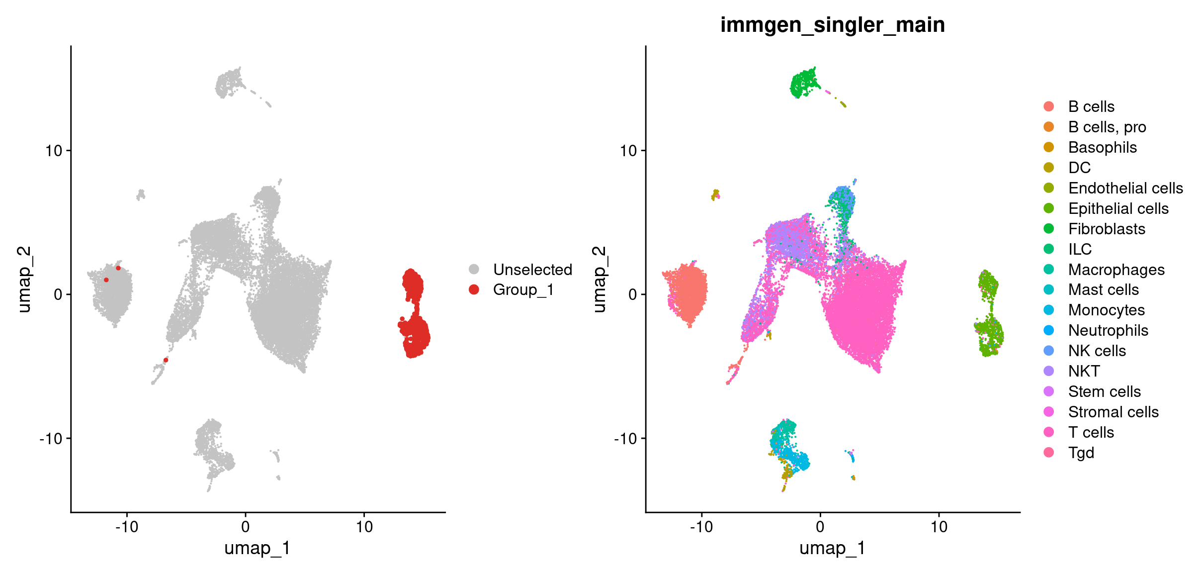
Looks like most of our tumor cells based on the CNV classification are in the epithelial cells cluster as we’d expect! A key point about CONICSmat here is that, the tool itself doesn’t determine a tumor cell from a non-tumor cell. In this case we knew from the whole genome data that the tumor cells should have gains in chromosomes 2 and 11 and a loss in chromosome 12. But if we did not have that information, we can overlay our celltypes on the heatmap and determine CNAs as the CNAs should primarily arise in the tumor’s celltype.
# using the celltypes argument we can add celltypes to the Seurat object.
plotHistogram(l[,candRegions_800],conicsmat_expr,clusters=3,zscoreThreshold=4, celltypes = merged_subset$immgen_singler_main)
#note that we got the cell barcodes from merged_subset as that
#was the object used to generate the initial conicsmat_expr matrix.
dev.off() #(after viewing)
We will look into adding this information to the Seurat object after we have the SNV tumor calls as well.
Finding tumor cells based on mutation data
We will use VarTrix to identify cells with mutations in our scRNAseq data. However, VarTrix is a tool that is run at the commandline level, so we will not run it in this workshop, instead we will go over the command to run it and how the outputs were processed here, and then plot the resulting mutation calls in RStudio. As input, VarTrix takes the scRNAseq BAM and barcodes.tsv files output from CellRanger, along with a VCF file containing the variants, and a reference genome fasta file. It can be run in 3 --scoring-method modes, here we chose coverage. This mode generates 2 output matrices- the ref-matrix and out-matrix that are in a MatrixMarket format. The former summarizes the number of REF reads (reads with wild-type allele) observed for every cell barcode and variant, while the latter summarizes the same for ALT reads (reads with mutant allele). Even though we will not be running it in this workshop, the vartrix command below was run for each replicate separately.
vartrix --vcf [input VCF file (based on cell line, is common for all replicates)] \
 --bam [cellranger bam file (unique to each replicate)] \
 --fasta [mm10 mouse reference genome] \
 --cell-barcodes [barcodes.tsv (unique to each replicate)] \
 --out-matrix [name of output ALT reads matrix] \
 --ref-matrix [name of output REF reads matrix] \
 --out-variants [name of output summarizing variants] -s coverage
The first few lines of one of the output matrices are shown below (both matrices are formatted the same way), where the first row summarizes the data so that the first value is the number of variants, second value is the number of cells, and the 3rd number is the number of rows in this matrix. The data itself starts from the 4th row, where the first column identifies the variant number (or ID), the second column identifies the cell barcode, and the third column indicates the number of reads (REF or ALT depending on the matrix) for that variant-
%%MatrixMarket matrix coordinate real general
% written by sprs
10427 4016 287647
3 359 0
3 890 0
3 1018 0
3 1068 0
3 1964 0
3 2048 0
...
The processing of these matrices to identify variant containing cells depends on the data. In the manuscript, the mutation calls were noisy, so the authors required a cell to have at least 2 variants with greater than 20X total coverage, with at least 5 ALT reads, and 10% VAF (variant allele fraction). However, if one has a confident set of tumor specific variants, the criteria to classify tumor specific cells can be less stringent. Here we will try two different approaches to filtering variants- first we will use the same list of variants the authors did and gradually increase the number of ALT reads we require to classify a cell as a tumor cell. Second, we will filter the original set of variants to a ‘higher confidence’ set of variants and classify tumor cells based on them. This section is also computationally intensive, so we will clear our workspace using the broom icon on the top right pane, and also click on the drop-down menu with a piechart beside it and select Free unused memory.
#Load libraries and packages if they are not loaded already
library(Seurat)
library(dplyr)
library(Matrix)
library(ggplot2)

#read in seurat object
merged <- readRDS(file='data/single_cell_rna/backup_files/preprocessed_object.rds')

#read in the variants file
variants_file <- read.csv('/cloud/project/data/single_cell_rna/cancer_cell_id/mcb6c-exome-somatic.variants.annotated.clean.filtered_10K.tsv', sep='\t')

#read in a sample's output VarTrix matrix and barcodes
##to read a sparse VarTrix matrix into R for processing, we'll use the readMM function, convert that to a matrix, and then convert the matrix to a dataframe.
rep1_icb_df <- as.data.frame(as.matrix(readMM('/cloud/project/data/single_cell_rna/cancer_cell_id/Rep1_ICB_alt_counts.mtx')))
##read in sample barcodes file
rep1_icb_bc <- read.table('/cloud/project/data/single_cell_rna/cancer_cell_id/Rep1_ICB_barcodes.tsv', sep = '\t', header = FALSE, col.names = 'barcodes')
Let’s spend some time looking at the variants_file, rep1_icb_bc and rep1_icb_df files. The variants_file was an output of our variant calling pipeline that uses 4 variant callers and includes some general variants filtering along with information like allele depth, allele fraction, etc. about each variant. The rep1_icb_bc file is a simple file containing all the barcodes in that sample. Lastly, the rep1_icb_df file is the matrix from earlier processed into a dataframe. You might be wondering how you are supposed to know how the matrix should be processed- usually most tools have (or at least should have) vignettes or brief tutorials available on how to process their data. Luckily for us, VarTrix does have all this documented in their GitHub documentation. So, let’s go through their website and see how they want us to process their data. Looks like after we read in the matrix, they want us to assign the barcodes as column names, and variants as row names. And after that we can look into adding that to our Seurat object. We have the barcodes in the rep1_icb_bc file, but what about the variants? We have the variant_file but it has chromosome and position separately, so we will make a column where they are combined together, and then add them to the matrix file.
#make a concatenated column of chromosome and variants
variants_file$CHROM_POS <- paste0(variants_file$CHROM, '_', variants_file$POS)
#assign barcodes to columns and variants to rows
colnames(rep1_icb_df) <- rep1_icb_bc$barcodes
row.names(rep1_icb_df) <- variants_file$CHROM_POS
#Hmm we got an error complaining about duplicate row names... that makes sense, since dataframes use the rownames to index a row,
#2 rows having the same index is a problem because it'll be an ambiguous index value.
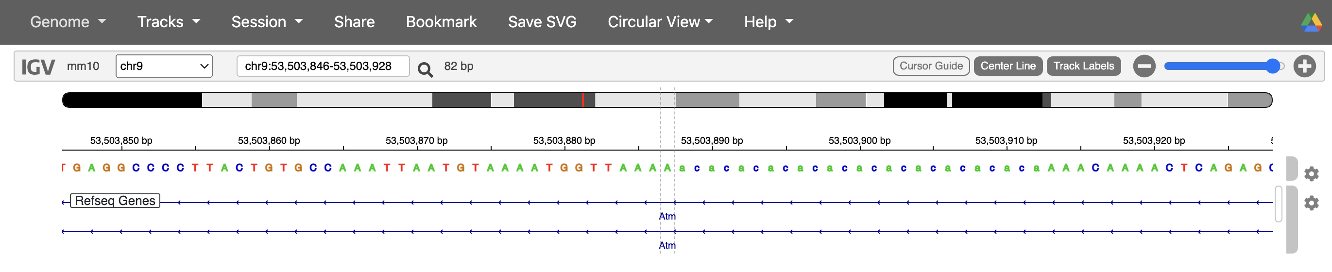
#But why do we have 2 occurrences of the same variant and does it happen multiple times? Luckily it told us one of the values where it ran into this error `chr9_53503887`.
#So let's look for it in the variant file. Interesting, we have 2 variants coming from the same position, it's difficult to say what's happening from the variant information alone, so we'll check what might be happening on IGV.
#For now, at least we know where the error is coming from. Let's check if there are any other similar occurrences.
#use the data.frame() and table() functions to get a dataframe summarizing the number of times each CHROM_POS value occurs
troubleshoot_df <- data.frame(table(variants_file$CHROM_POS))
#sort or order the dataframe in descending order of occurrences for ease of viewing
troubleshoot_df <- troubleshoot_df[order(troubleshoot_df$Freq, decreasing = TRUE),]
#look at the top 5 rows
head(troubleshoot_df)
#looks like it only happens once!
#We can get around this error by using the make.unique() function in R.
#This function goes through a column and for any values that occur more than once, it appends `_` and a number to the value.
variants_file$CHROM_POS <- make.unique(as.character(variants_file$CHROM_POS), sep = "_")
#navigate through the dataframe and see what changed.
#Okay now let's try assign the variants to a row again
row.names(rep1_icb_df) <- variants_file$CHROM_POS
#Success!
While it’s difficult to say what exactly happened in the case of the variant at chr9_53503887 without loading this sample’s BAM file into IGV, based on the reference genome, one possibility is that due to the variant being in a soft-masked/ repetitive region, the alignment algorithms were not able to align the reads well and so we have some instances where it was called as 4 base deletion, and others where it was called as a 2 base deletion.
Let’s look at this dataframe more carefully now. So we have a dataframe with cell barcodes as columns and variants as rows. And each cell or value in this dataframe is the number of ALT reads (aka reads containing a mutation). Our overall objective is to find tumor cells, and we want to do that by establishing some sort of a threshold of number of ALT reads needed for a cell to be a tumor cell. Now we can do that for every sample separately or make a superset dataframe and do all the filtering together. The second approach might be better because eventually our goal is to combine cells from all the samples with the Seurat object. In order to make a superset dataframe, first we need to do the above formatting for each vartrix output. Then, we can combine the results horizontally because we need to add the cell barcodes. The key to combining dataframes horizontally is that the rownames (or index) need to be the same, and that is the case here because we ran Vartrix for all samples using the same set of variants.
#first let's make a vector of samples
sample_names <- c('Rep1_ICB', 'Rep1_ICBdT', 'Rep3_ICB', 'Rep3_ICBdT', 'Rep5_ICB', 'Rep5_ICBdT')

# Initialize an empty dataframe with the rows predefined as variant_names
all_samples_vartrix_df <- data.frame(matrix(nrow = length(variants_file$CHROM_POS), ncol = 0))
rownames(all_samples_vartrix_df) <- variants_file$CHROM_POS

#Now loop through each sample in sample_names and format them using the code from before
for (sample_rep in sample_names) {
  #read in and processing a sparse matrix
  rep_df <- data.frame(as.matrix(readMM(paste0('/cloud/project/data/single_cell_rna/cancer_cell_id/', sample_rep, '_alt_counts.mtx'))))

  #get each sample's barcodes
  rep_bc <- read.table(paste0('/cloud/project/data/single_cell_rna/cancer_cell_id/', sample_rep, '_barcodes.tsv'),
    sep = '\t', header = FALSE, col.names = 'barcodes')

  #set column names and row names
  colnames(rep_df) <- rep_bc$barcodes
  row.names(rep_df) <- variants_file$CHROM_POS

  #combine dataframes
  all_samples_vartrix_df <- cbind(all_samples_vartrix_df, rep_df)
}

#let's double check that the number of columns make sense.
#the number of cell barcodes in each of our replicates should be the same as the number of columns in all_samples_vartrix_df
#number of columns in dataframe
ncol(all_samples_vartrix_df) #28585
#number of rows in each sample's dataframe # 4016+3927+6390+5576+2828+5848
#have a variable that we'll keep adding the number of rows to
tracking_sum = 0
#loop through each sample and count the number of rows in that dataframe.
#Add that value to the tracking_sum value, and also print the row every time.
for (sample_rep in sample_names) {
  rep_bc <- read.table(paste0('/cloud/project/data/single_cell_rna/cancer_cell_id/', sample_rep, '_barcodes.tsv'), sep = '\t', header = FALSE, col.names = 'barcodes')
  print(nrow(rep_bc))
  tracking_sum <- tracking_sum + nrow(rep_bc)
}

#print the tracking sum and compare to the value we got from ncol
print(tracking_sum)
Now we have all the cells in one dataframe, with information about the number of ALT reads for each variant. Next, we can get to classifying some tumor cells. For this, we’ll first want to flip (or transpose) the matrix so that the cell barcodes are on the rows and variants are on the columns. The reason for this will become clearer soon, but basically we need to know the number of total ALT reads across all variants in each cell, and the way dataframe operations work, it is much easier to do that by adding a column and take the sum off all the values in the row. To transpose the dataframe, we can use a handy R function called t(). And then we can take the sum of values in the dataframe using rowSums(). Once we have that, we can start subsetting the dataframe and making UMAP plots that highlight cells depending on how many ALT reads we want to require for a cell to be considered a tumor cell.
#transpose the dataframe
all_samples_vartrix_df <- as.data.frame(t(all_samples_vartrix_df))
#The t() function technically outputs a matrix and that needs to be converted to a dataframe

#this is a large matrix and ends up being computationally heavy so run the following command
gc() #this is the same as 'free unused R memory'

#now let's add a column that is the sum of the entire row so that we can see the number of ALT reads per cell
all_samples_vartrix_df$num_alt_reads <- rowSums(all_samples_vartrix_df)

#Now let's highlight cells in Seurat with at least 1 ALT read
## first get a dataframe where everything has at least 1 ALT read using that column we added
all_samples_vartrix_df_1_ALT_read <- all_samples_vartrix_df[all_samples_vartrix_df$num_alt_reads >= 1,]
DimPlot(merged, cells.highlight = rownames(all_samples_vartrix_df_1_ALT_read)) +
  ggtitle('UHighlighting cells with \nat least 1 ALT read')
#that's way too many 'tumor' cells especially since we know a lot of the cells are not even epithelial cells.

#Let's try this again but increase our requirement to 10 ALT reads.
#Also, we don't need to make a new dataframe every time, we can load the cells.highlight directly from the all_sample_vartrix_df table
DimPlot(merged, cells.highlight = rownames(all_samples_vartrix_df[all_samples_vartrix_df$num_alt_reads >= 10,])) +
  ggtitle('Highlighting cells with \nat least 10 ALT reads')

#That seems to have helped, but we're still getting a lot more cells than we'd expect
#considering that the epithelial cells are largely in clusters 9 and 12
#let's increase the number of ALT reads up to 20
DimPlot(merged, cells.highlight = rownames(all_samples_vartrix_df[all_samples_vartrix_df$num_alt_reads >= 20,])) +
  ggtitle('Highlighting cells with \nat least 20 ALT reads')
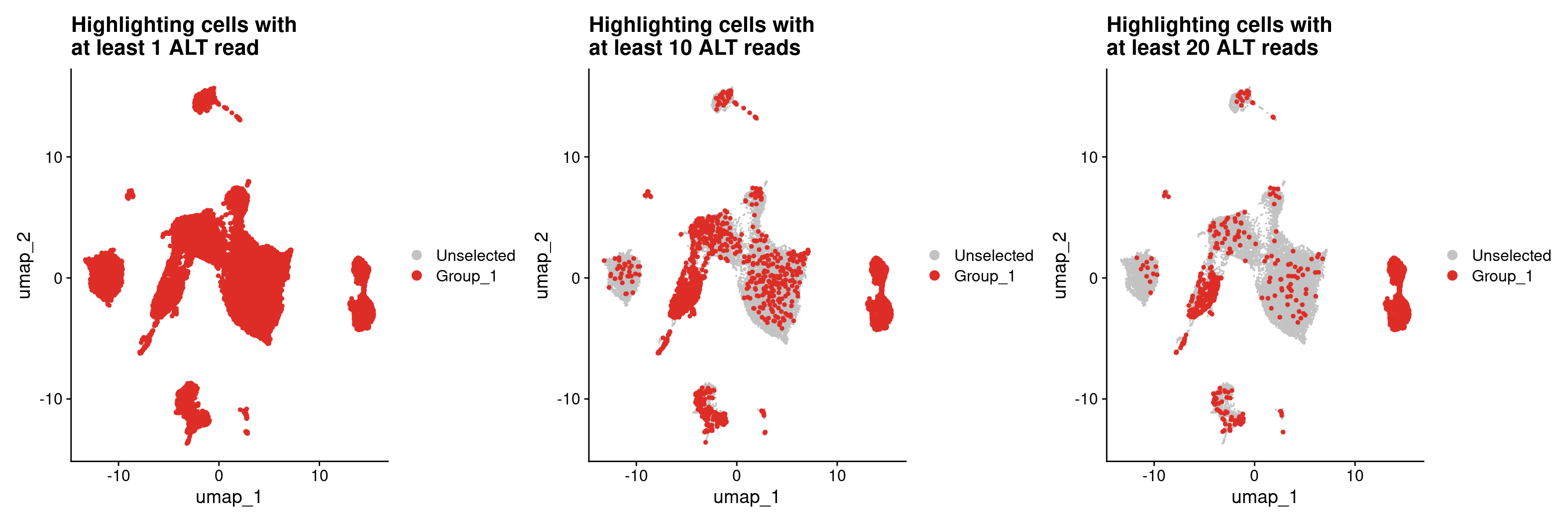
In spite of being fairly strict with how we are defining a tumor cell by requiring at least 20 reads carrying a mutation for a cell to be a tumor cell, we are still getting some pretty noisy calls as we are identifying many cells that are unlikely to be epithelial cells as tumor cells. This could suggest that our original variant list was not filtered enough and still has germline variants. We can filter this variant file further by removing variants that are likely to be germline variants using the following filtering strategy.
# Before we move forward let's delete some files and free up some space
rm(rep1_icb_bc, rep1_icb_df, troubleshoot_df, all_samples_vartrix_df_1_ALT_read)
gc()

# Filter variants file to high confidence variants
variants_file_high_conf <- variants_file[variants_file$set == 'mutect-varscan-strelka' &
                           variants_file$NORMAL.DP > 50 &
                           variants_file$TUMOR.DP > 50 &
                           variants_file$NORMAL.AF < 0.01 &
                           variants_file$TUMOR.AF > 0.25 &
                           variants_file$Consequence == 'missense_variant', ]
What are these filters doing?
- The
setcolumn only keeps variants that were called by all 3 mutation callers (mutect, varscan, and strelka). - (
NORMAL.DP) and (TUMOR.DP) require that there at least 50 reads of support of the variant position in both the tumor and normal samples. NORMAL.AFfilter requires that if a variant does occur in the normal sample, it is at a VAF of less than 1%.TUMOR.AFfilter requires that a variant occurs in the tumor sample at at least 25% VAF.CONSEQUENCEdictates that we only look at missense mutations.
Let’s use this high confidence variants file, restrict our superset variants matrix to this list of variants. And see if this works better to classify tumor cells.
#get a list of high confidence variants
high_conf_variants <- variants_file_high_conf$CHROM_POS
#the list of variants corresponds to the columns of our dataframe,
#so we can use the list of high_conf_variants as a list of columns to keep in our dataframe
all_samples_vartrix_df_high_conf <- all_samples_vartrix_df[high_conf_variants]
#now let's recalculate num_alt_reads based on these ~2K high confidence variants
all_samples_vartrix_df_high_conf$num_alt_reads <- rowSums(all_samples_vartrix_df_high_conf)
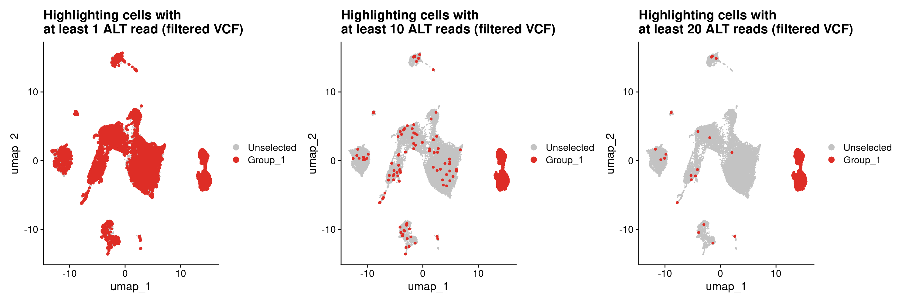
#let's plot potential tumor cells based on the high confidence variants using the same thresholds as before.
#At least 1 ALT read for a tumor cell
DimPlot(merged, cells.highlight = rownames(all_samples_vartrix_df_high_conf[all_samples_vartrix_df_high_conf$num_alt_reads >= 1,])) +
ggtitle('Highlighting cells with \nat least 1 ALT read (filtered VCF)')
#At least 10 ALT reads for a tumor cell
DimPlot(merged, cells.highlight = rownames(all_samples_vartrix_df_high_conf[all_samples_vartrix_df_high_conf$num_alt_reads >= 10,])) +
ggtitle('Highlighting cells with \nat least 10 ALT reads (filtered VCF)')
#At least 20 ALT reads for a tumor cell
DimPlot(merged, cells.highlight = rownames(all_samples_vartrix_df_high_conf[all_samples_vartrix_df_high_conf$num_alt_reads >= 20,])) +
ggtitle('Highlighting cells with \nat least 20 ALT reads (filtered VCF)')
#How does this compare against our previous plot?
tumor_cells_10Kvars_dimplot <- DimPlot(merged, cells.highlight = rownames(all_samples_vartrix_df[all_samples_vartrix_df$num_alt_reads >= 20,])) +
ggtitle('Tumor cells with at least 20 ALT reads \n- 10K variants')
tumor_cells_2Kvars_dimplot <- DimPlot(merged, cells.highlight = rownames(all_samples_vartrix_df_high_conf[all_samples_vartrix_df_high_conf$num_alt_reads >= 20,])) +
ggtitle('Tumor cells with at least 20 ALT reads \n- 2K variants')
## Plot them side by side
tumor_cells_10Kvars_dimplot + tumor_cells_2Kvars_dimplot
#That looks way better! Based on this, I think we can be pretty happy about finding tumor cells from the high confidence variants
all_samples_vartrix_df_high_conf_20_ALT_read <- all_samples_vartrix_df_high_conf[all_samples_vartrix_df_high_conf$num_alt_reads >= 20,]
snv_tumor_bc <- rownames(all_samples_vartrix_df_high_conf_20_ALT_read)
write.table(x = snv_tumor_bc, file = 'outdir_single_cell_rna/snv_tumor_bc_list.tsv', row.names = FALSE, col.names = 'snv_tumor_barcodes', quote=FALSE)
Lastly, let’s look into adding the SNV and CNV based tumor cell classifications to our Seurat object’s metadata. To add metadata to a Seurat object, we need a dataframe where we have all the barcodes in the Seurat object as rownames, and column(s) that we want to add to the metadata with value(s) corresponding to each barcode. Recall that our tumor cell classification lists for both SNVs and CNVs include only the tumor cell barcodes. So we will need a list of all barcodes in the Seurat object.
#read in our CNV and SNV tumor cell classification files
snv_bc_df <- read.csv('outdir_single_cell_rna/snv_tumor_bc_list.tsv', sep='\t')
cnv_bc_df <- read.csv('outdir_single_cell_rna/cnv_tumor_bc_list.tsv', sep='\t')

# If R crashed before you got to these steps, we have backip
# snv_bc_df <- read.csv('data/single_cell_rna/backup_files/snv_tumor_bc_list.tsv', sep='\t')
# cnv_bc_df <- read.csv('data/single_cell_rna/backup_files/cnv_tumor_bc_list.tsv', sep='\t')

#get lists of these barcodes
snv_bc_list <- snv_bc_df$snv_tumor_barcodes
cnv_bc_list <- cnv_bc_df$cnv_tumor_barcodes

#read in our Seurat object (if it's not already in your environment)
merged <- readRDS('outdir_single_cell_rna/preprocessed_object.rds')

#get all barcodes from our Seurat object
all_bc <- rownames(merged@meta.data)
#convert them into a dataframe
all_bc_df <- data.frame(all_bc)
#add 2 columns that will hold the SNV tumor cell classifications (snv_class) and #CNV tumor cell classifications (cnv_class) prefilled with the value 'unclassified'
all_bc_df$snv_class <- 'unclassified'
all_bc_df$cnv_class <- 'unclassified'

#for barcodes in each of our SNV and CNV lists,
#we'll change the value in the corresponding columns to 'snv_tumor' and 'cnv_tumor'
all_bc_df$snv_class[all_bc_df$all_bc %in% snv_bc_list] <- 'snv_tumor'
all_bc_df$cnv_class[all_bc_df$all_bc %in% cnv_bc_list] <- 'cnv_tumor'

#now let's add these classifications to Seurat metadata
#first we need to make the barcodes column as the rownames or index and delete the extra column.
rownames(all_bc_df) <- all_bc_df$all_bc
#open the all_bc_df and see what happened. We don't need the extra barcodes column, so let's get rid of that.
all_bc_df$all_bc <- NULL
#finally, let's add this to the Seurat metadata using Seurat's AddMetaData function
merged <- AddMetaData(merged, all_bc_df)
#see what columns were added to the metadata column
colnames(merged@meta.data)

#Now let's plot the CNV and SNV classifications on our UMAP
DimPlot(merged, group.by = c('snv_class', 'cnv_class', 'immgen_singler_main'))

#let's also take a quick look at how much the snv and cnv classifications agree with each other
table(merged$cnv_class, merged$snv_class)
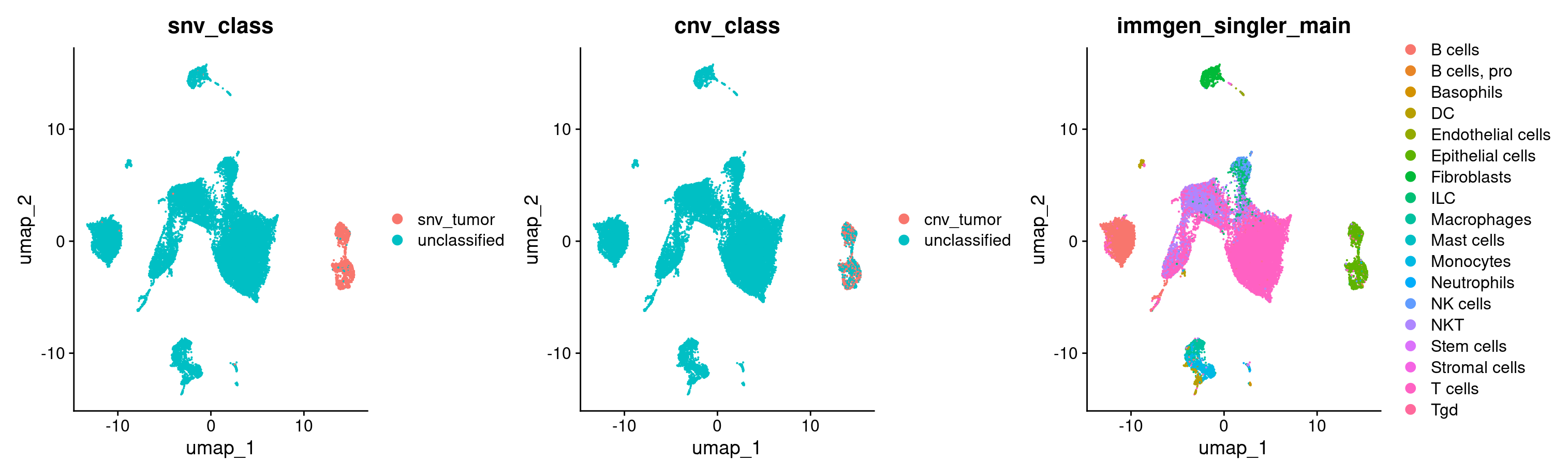
> table(merged$cnv_class, merged$snv_class)
               snv_tumor unclassified
  cnv_tumor          822           12
  unclassified       495        21856
Voila! Looks like both of our independent classifications of tumor cells agree to quite a large extent. They also both independently added to our tumor cell identification, and were restricted to the epithelial cells.