Differential expression analysis
In this section we will use the previously generated Seurat object that has gone through the various preprocessing steps, clustering, and celltyping, and use it for gene expression and differential expression analyses. We will carry out two sets of differential expression analyses in this module. Firstly, since we know that the tumor cells should be epithelial cells, we will begin by trying to identify epithelial cells in our data using expression of Epcam as a marker. Subsequently, we will carry out a DE analysis within the Epcam-positive population(s). Secondly, we will compare the T cell populations of mice treated with ICB therapy against mice with their T cells depleted that underwent ICB therapy to determine differences in T cell phenotypes. We will also briefly explore pseudobulk differential expression analysis. Pseudobulk DE analysis may be more robust in situations where one is comparing conditions and has multiple replicates in their experiment.
Read-in the saved seurat object from the previous step if it is not already loaded in your current R session.
library(Seurat)
library(dplyr)
library(EnhancedVolcano)
library(presto)
merged <- readRDS('outdir_single_cell_rna/preprocessed_object.rds')

#alternatively we have a seurat object from the last step saved here if you need it.
merged <- readRDS('/cloud/project/data/single_cell_rna/backup_files/preprocessed_object.rds')
Gene expression analysis for epithelial cells
Use Seurat’s FeaturePlot function to color each cell by its Epcam expression on a UMAP.
FeaturePlot requires at least 2 arguments- the seurat object, and the ‘feature’ you want to plot (where a ‘feature’ can be a gene, PC scores, any of the metadata columns, etc.). To customize the FeaturePlot, please refer to Seurat’s documentation here
FeaturePlot(merged, features = 'Epcam')
While there are some Epcam positive cells scattered on the UMAP, there appear to be 2 clusters of cells in the UMAP that we may be able to pull apart as potentially being malignant cells.
There are a few different ways to go about identifying what those clusters are. We can start by trying to use the DimPlot plotting function from before along with the FeaturePlot function. Separating plots by the + symbol allows us to plot multiple plots side-by-side.
DimPlot(merged, group.by = 'seurat_clusters_res0.8', label = TRUE) +
FeaturePlot(merged, features = 'Epcam') +
DimPlot(merged, group.by = 'immgen_singler_main')
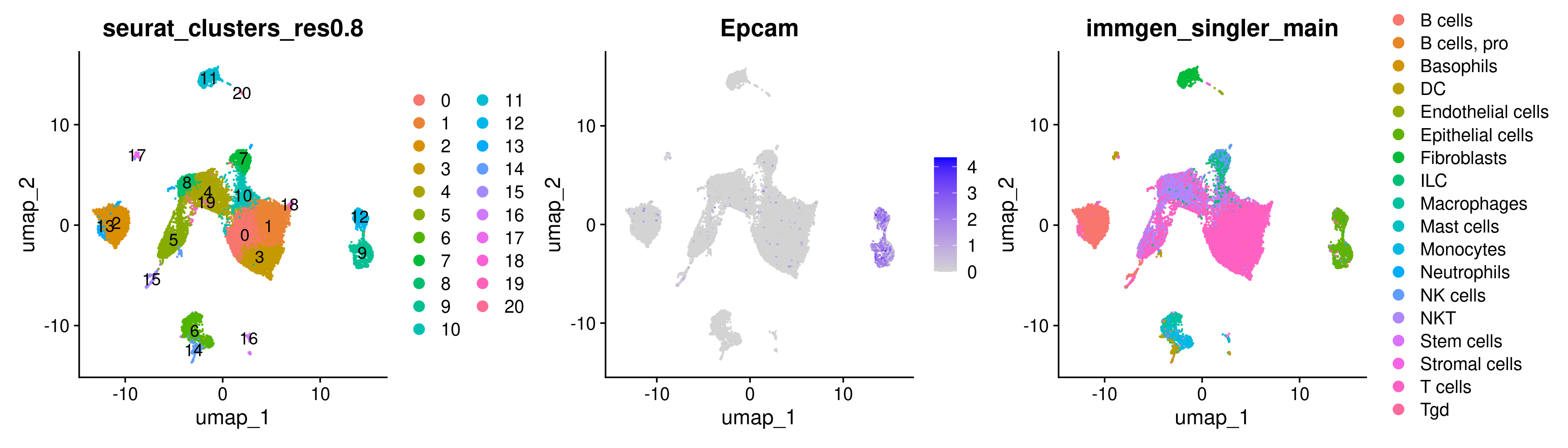
While the plots generated by the above commands make it pretty clear that the clusters of interest are clusters 9 and 12, sometimes it is trickier to determine which cluster we are interested in solely from the UMAP as the clusters may be overlapping. In this case, a violin plot VlnPlot may be more helpful. Similar to FeaturePlot, VlnPlot also takes the Seurat object and features as input. It also requires a group.by argument that determines the categorical variable that will be used to group the cells.
To learn more about customizing a Violin plot, please refer to the Seurat documentation
VlnPlot(merged, group.by = 'seurat_clusters_res0.8', features = 'Epcam')
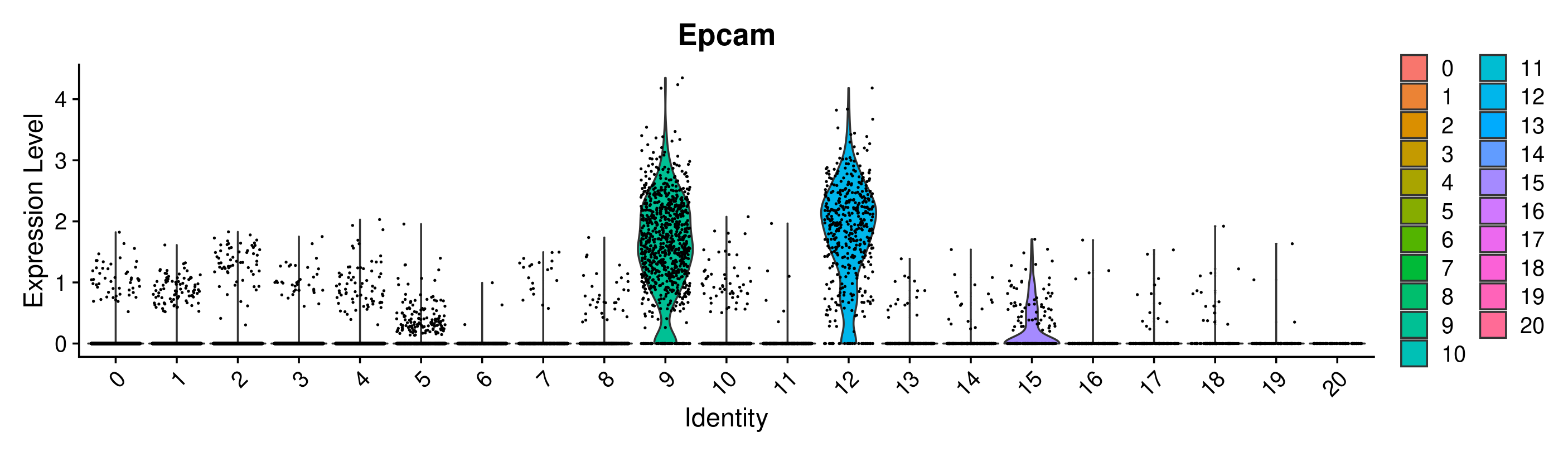
Great! Looks like we can confirm that clusters 9 and 12 have the highest expression of Epcam. However, it is interesting that they are split into 2 clusters. This is a good place to use differential expression analysis to determine how these clusters differ from each other.
Differential expression for epithelial cells
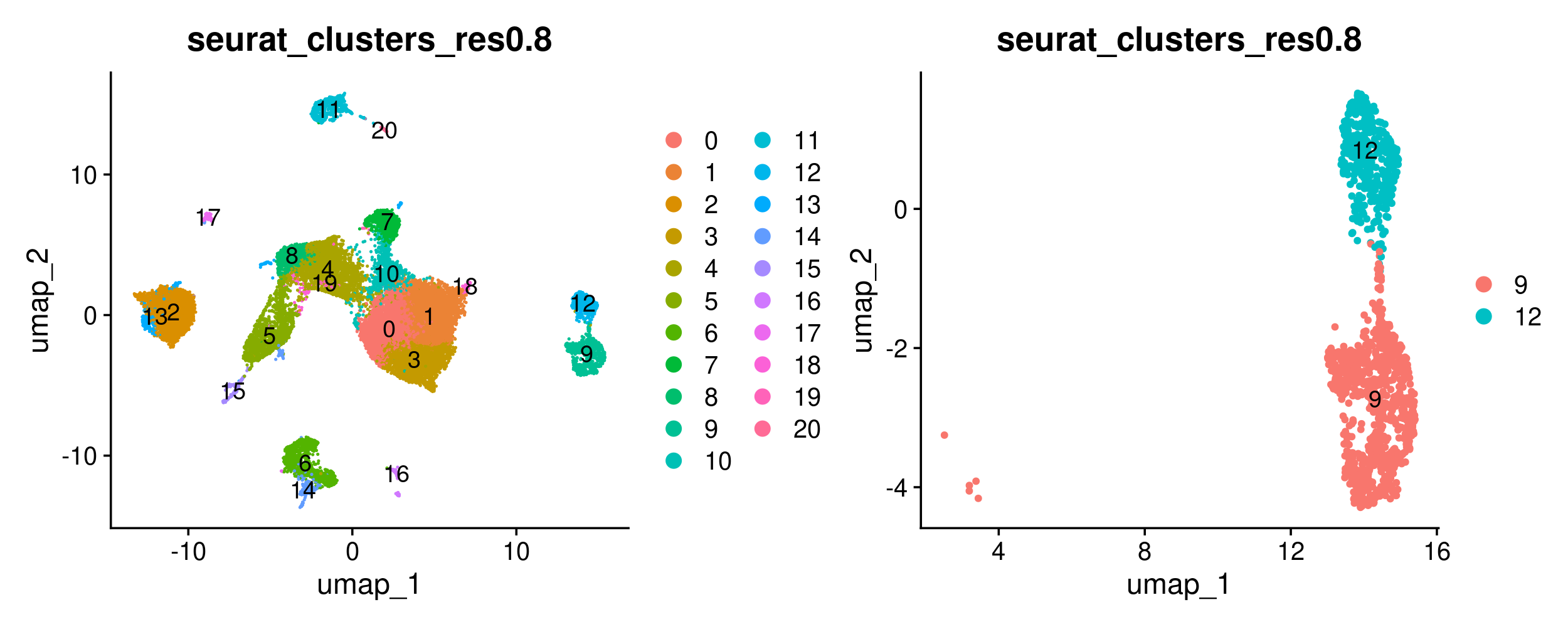
We can begin by restricting the Seurat object to the cells we are interested in. We will do so using Seurat’s subset function, that allows us to create an object that is filtered to any values of interest in the metadata column. However, we first need to set the default identity of the Seurat object to the metadata column we want to use for the ‘subset’, and we can do so using the SetIdent function. After subsetting the object, we can plot the original object and subsetted object side-by-side to ensure the subsetting happened as expected. We can also count the number of cells of each type to confirm the same.
#set ident to seurat clusters metadata column and subset object to Epcam positive clusters
merged <- SetIdent(merged, value = 'seurat_clusters_res0.8')
merged_epithelial <- subset(merged, idents = c('9', '12'))

#confirm that we have subset the object as expected visually using a UMAP
DimPlot(merged, group.by = 'seurat_clusters_res0.8', label = TRUE) +
DimPlot(merged_epithelial, group.by = 'seurat_clusters_res0.8', label = TRUE)

#confirm that we have subset the object as expected by looking at the individual cell counts
table(merged$seurat_clusters_res0.8)
table(merged_epithelial$seurat_clusters_res0.8)
Now we will use Seurat’s FindMarkers function to carry out a differential expression analysis between both groups. FindMarkers also requires that we use SetIdent to change the default ‘Ident’ to the metadata column we want to use for our comparison. More information about FindMarkers is available here.
Note that here we use FindMarkers to compare clusters 9 and 12. The default syntax of FindMarkers requires that we provide each group of cells as ident.1 and ident.2. The output of FindMarkers is a table with each gene that is differentially expressed and its corresponding log2FC. The direction of the log2FC is of ident.1 with respect to ident.2. Therefore, genes upregulated in ident.1 have positive log2FC, while those downregulated in ident.1 have negative log2FC. The min.pct=0.25 argument tests genes that are expressed in 25% of cells in either of the ident.1 or ident.2 groups. This can help reduce false positives as the genes must be expressed in a greater proportion of the cells compared to the default value of 1%. The logfc.threshold=0.1 parameter ensures our results only include genes that have a fold change of less than -0.1 or more than 0.1. Increasing the min.pct and logfc.threshold parameters can also result in the function running faster by reducing the number of genes being tested.
#carry out DE analysis between both groups
merged_epithelial <- SetIdent(merged_epithelial, value = "seurat_clusters_res0.8")
epithelial_de <- FindMarkers(merged_epithelial, ident.1 = "9", ident.2 = "12", min.pct=0.25, logfc.threshold=0.1) #how cluster 9 changes wrt cluster 12
On opening epithelial_de in your RStudio session, you’ll see that it is a dataframe with the genes as rownames, and the following columns- p_val, avg_log2FC, pct.1, pct.2, p_val_adj. The p-values are dependent on the test used while running FindMarkers, and the adjusted p-value is based on the bonferroni correction test. pct.1 and pct.2 are the percentages of cells where the gene is detected in the ident.1 and ident.2 groups respectively.
Next we can subset this dataframe to only include DE genes that have a significant p-value, and then further subset the ‘significant DE genes only’ dataframe to the top 20 genes with the highest absolute log2FC. Looking at the absolute log2FC allows us to capture both, upregulated and downregulated genes.
#restrict differentially expressed genes to those with an adjusted p-value less than 0.001
epithelial_de_sig <- epithelial_de[epithelial_de$p_val_adj < 0.001,]

#get the top 20 genes by fold change
epithelial_de_sig_top20 <- epithelial_de_sig %>%
  top_n(n = 20, wt = abs(avg_log2FC))
epithelial_de_sig_top20 is a dataframe that is restricted to the top20 most differentially expressed genes by log2FC.
There are a few ways we can visualize the differentially expressed genes. We’ll start with the Violin and Feature plots from before. We can also visualize DEs using a DotPlot that allows us to capture both the average expression of a gene and the % of cells expressing it. In addition to these in-built Seurat functions, we can also generate a volcano plot using the EnhancedVolcano package. For the volcano plot, we can use the unfiltered DE results as the function colors and labels genes based on parameters (pCutoff, FCcutoff) we specify.
#get list of top 20 DE genes for ease
epithelial_de_sig_top20_genes <- rownames(epithelial_de_sig_top20)

#plot all 20 genes in violin plots
VlnPlot(merged_epithelial, features = epithelial_de_sig_top20_genes,
  group.by = 'seurat_clusters_res0.8', ncol = 5, pt.size = 0)

#plot all 20 genes in UMAP plots
FeaturePlot(merged_epithelial, features = epithelial_de_sig_top20_genes, ncol = 5)

#plot all 20 genes in a DotPlot
DotPlot(merged_epithelial, features = epithelial_de_sig_top20_genes,
  group.by = 'seurat_clusters_res0.8') + RotatedAxis()

#plot all differentially expressed genes in a volcano plot
EnhancedVolcano(epithelial_de,
  lab = rownames(epithelial_de),
  x = 'avg_log2FC',
  y = 'p_val_adj',
  title = 'Cluster9 wrt Cluster 12',
  pCutoff = 0.05,
  FCcutoff = 0.5,
  pointSize = 3.0,
  labSize = 5.0,
  colAlpha = 0.3)
To find out how we can figure out what these genes mean, stay tuned! The next module on pathway analysis will help shed some light on that. For now, let’s create a TSV file containing our DE results for use later on. We will need to rerun FindMarkers with slightly different parameters for this- we will change the logfc.threshold parameter to 0, as one of the pathway analysis tools requires all genes to be included in the analysis (more on that later).
#rerun FindMarkers
epithelial_de_gsea <- FindMarkers(merged_epithelial, ident.1 = "9",
  ident.2 = "12", min.pct=0.25, logfc.threshold=0)
#save this table as a TSV file (first move index to first column)
epithelial_de_gsea <- tibble::rownames_to_column(epithelial_de_gsea, var = "gene")
write.table(x = epithelial_de_gsea, file = 'outdir_single_cell_rna/epithelial_de_gsea.tsv', sep='\t', row.names = FALSE)
Classic single-cell based differential expression analysis is notorious for having a high number of false positives. This has been attributed to a few reasons such as each cell being considered an independent observation resulting in inflated p-values and it not taking replicates into account. Psuedobulk based differential expression analyses can be incorporated to at least in part get around these (Junttila S, Smolander J, et al. (2022); Squair, J.W. et al. (2021)).
Depending on the type of experiment, you’re unlikely to always have replicates, but here we do, therefore, we will carry out a pseudobulk DE analysis and compare the results against our conventional single-cell DE analysis. The first step is to generate a pseudobulk Seurat object using Seurat’s in-built function AggregateExpression, more information on the function is available here and Seurat’s pseudobulk DE vignette is here. The function makes groups based on the metadata columns we specify, sums the counts for each gene within the group, and then log normalizes and scales the data. The resulting object is structured like our single-cell Seurat object with different layers for the raw counts (counts), log normalized (data) and scaled (scale.data) data. However, instead of the rows being our cell barcodes, they are a combination of the grouping categories we used as an input. Here, we will use the sample (given by orig.ident) as our replicates and the differential expression analysis will use DESeq2 to compare clusters 9 and 12. Specifying DESeq2 in the test.use argument will allow us to use Seurat’s implementation of DESeq2. There are quite a few other tests that can be used, we primarily chose DESeq2 here because it was in Seurat’s DE vignette linked previously, but we encourage you to look into the various other tests as well.
# Aggregate counts for each sample and cluster combination
pb_epithelial <- AggregateExpression(merged_epithelial, assays = 'RNA',
                                         return.seurat = T, group.by = c('orig.ident', 'seurat_clusters_res0.8'))
# See the first few rows of the log normalized data layer
print(head(pb_epithelial@assays$RNA$data))

#Change ident to seurat clusters
Idents(pb_epithelial) <- "seurat_clusters_res0.8"

# Use FindMarkers with DESeq2 as the test to compare cluster 9 wrt cluster 12
pb_epithelial_de <- FindMarkers(object = pb_epithelial, test.use = "DESeq2",
                              ident.1 = "9", ident.2 = "12")


# The DESeq2 analysis results in NAs in the pvalue columns for some cases
pb_epithelial_de <- na.omit(pb_epithelial_de)

# Restrict differentially expressed genes to those with an adjusted p-value less than 0.001
pb_epithelial_de_sig <- pb_epithelial_de[pb_epithelial_de$p_val_adj < 0.01,]


# Compare significantly differentially expressed genes
pb_and_sc_genes <- intersect(rownames(epithelial_de_sig), rownames(pb_epithelial_de_sig))
only_sc_genes <- setdiff(rownames(epithelial_de_sig), rownames(pb_epithelial_de_sig))
only_pb_genes <- setdiff(rownames(pb_epithelial_de_sig), rownames(epithelial_de_sig))

print(paste0("Genes differentially expressed in both single-cell and pseudobulk: ", length(pb_and_sc_genes)))
print(paste0("Genes differentially expressed in single-cell but not pseudobulk: ", length(only_sc_genes)))
print(paste0("Genes differentially expressed in pseudobulk but not single-cell: ", length(only_pb_genes)))
Genes that were detected by single-cell and pseudobulk (~2800) are the most likely to be true positives. Far fewer genes are detected by pseudobulk only (~600) compared to single-cell only (~3000). The pseudobulk genes may also be false positives though, as by pseudobulking we lose information about the percent of cells expressing the genes. Therefore, some of these genes may be differentially expressed because they are only expressed in a few cells. Also, it is unlikely that all ~3000 genes detected only by single-cell are false positives- therefore, it’s difficult to advocate for only one approach, but based on the downstream application one approach may be better than the other. (If the goal is to come up with a shorter list of genes to follow up on in the wet lab, then the consensus DE gene list may be appropriate. But if the goal is more exploratory, the single cell genes can be used, but you’ll likely want to use violin plots and feature plots to make sure the genes are indeed differentially expressed).
Differential expression for T cells
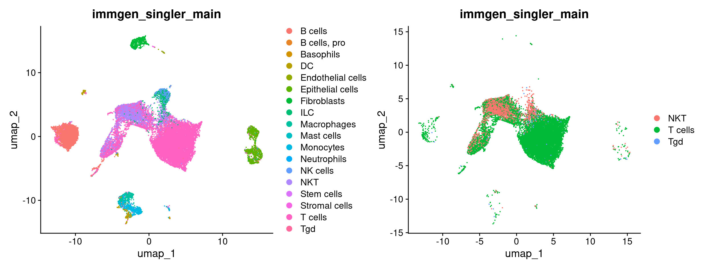
For the T cell focused analysis, we will ask how T cells from mice treated with ICB compare against T cells from mice with (some of) their T cells depleted treated with ICB (ICBdT). We will start by subsetting our merged object to only have T cells, by combining the various T cell annotations from celltyping section. We’ll start by seeing all the possible celltypes we have, and picking the ones that are related to T cells. Next, we will SetIdent to the celltype metadata column, and subset to the celltypes that correspond to T cells. Finally, we’ll doublecheck that the subsetting happened as we expected it to.
#check all the annotated celltypes
unique(merged$immgen_singler_main)

#pick the ones that are related to T cells
t_celltypes_names <- c('T cells', 'NKT', 'Tgd')
merged <- SetIdent(merged, value = 'immgen_singler_main')
merged_tcells <- subset(merged, idents = t_celltypes_names)

#confirm that we have subset the object as expected visually using a UMAP
DimPlot(merged, group.by = 'immgen_singler_main') +
DimPlot(merged_tcells, group.by = 'immgen_singler_main')

#confirm that we have subset the object as expected by looking at the individual cell counts
table(merged$immgen_singler_main)
table(merged_tcells$immgen_singler_main)
Now we want to compare T cells from mice treated with ICB vs ICBdT. First, we need to distinguish the ICB and ICBdT cells from each other. Start by clicking on the object in RStudio and expand meta.data to get a snapshot of the columns and the what kind of data they hold.
We can leverage the orig.ident column again as it has information about the condition and replicates. For the purposes of this DE analysis, we want a meta.data column that combines the replicates of each condition. That is, we want to combine the replicates of each condition together into a single category (ICB vs ICBdT).
#we'll start by checking the possible names each replicate has.
unique(merged_tcells$orig.ident)

#there are 6 possible values, 3 replicates for the ICB treatment condition, and 3 for the ICBdT condition
#so we can combine "Rep1_ICB", "Rep3_ICB", "Rep5_ICB" to ICB, and "Rep1_ICBdT", "Rep3_ICBdT", "Rep5_ICBdT" to ICBdT.
#first initialize a metadata column for experimental_condition
merged_tcells@meta.data$experimental_condition <- NA

#Now we can take all cells that are in each replicate-condition,
#and assign them to the appropriate condition
merged_tcells@meta.data$experimental_condition[merged_tcells@meta.data$orig.ident %in% c("Rep1_ICB", "Rep3_ICB", "Rep5_ICB")] <- "ICB"
merged_tcells@meta.data$experimental_condition[merged_tcells@meta.data$orig.ident %in% c("Rep1_ICBdT", "Rep3_ICBdT", "Rep5_ICBdT")] <- "ICBdT"

#double check that the new column we generated makes sense
#(each replicate should correspond to its experimental condition)
table(merged_tcells@meta.data$orig.ident, merged_tcells@meta.data$experimental_condition)
With the experimental conditions now defined, we can compare the T cells from both groups. We’ll start by using FindMarkers using similar parameters to last time, and see how ICBdT changes with respect to ICB. Next, restrict the dataframe to significant genes only, and then look at the top 5 most upregulated and downregulated DE genes by log2FC.
#carry out DE analysis between both groups
merged_tcells <- SetIdent(merged_tcells, value = "experimental_condition")
tcells_de <- FindMarkers(merged_tcells, ident.1 = "ICBdT", ident.2 = "ICB", min.pct=0.25)

#restrict differentially expressed genes to those with an adjusted p-value less than 0.001
tcells_de_sig <- tcells_de[tcells_de$p_val_adj < 0.001,]

#find the top 5 most downregulated genes
tcells_de_sig %>%
  top_n(n = 5, wt = -avg_log2FC)
#find the top 5 most upregulated genes
tcells_de_sig %>%
  top_n(n = 5, wt = avg_log2FC)
The most downregulated gene in the ICBdT condition based on foldchange is Cd4. That makes sense, because the monoclonal antibody (GK1.5) used for T cell depletion specifically targets CD4 T cells! You can read more about the antibody here.
Interestingly, for the list of genes that are upregulated in the ICBdT condition, we see Cd8b1 show up. It could be interesting to see if the CD8 T cells’ phenotype changes based on the treatment condition. Let’s subset the object to CD8 T cells only, find DE genes to see how ICBdT CD8 T cells change compared to ICB CD8 T cells, and visualize these similar to before.
# Subset object to CD8 T cells. Since we already showed how to subset cells using the clusters earlier,
# This time we'll subset to CD8 T cells by selecting for cells with high expression of Cd8 genes and low expression of Cd4 genes using violin plots to find thresholds for filtering
VlnPlot(merged_tcells, features = c('Cd8a', 'Cd8b1', 'Cd4'))
merged_cd8tcells <- subset(merged_tcells, subset= Cd8b1 > 1 & Cd8a > 1 & Cd4 < 0.1)

#carry out DE analysis between both groups
merged_cd8tcells <- SetIdent(merged_cd8tcells, value = "experimental_condition")
cd8tcells_de <- FindMarkers(merged_cd8tcells, ident.1 = "ICBdT", ident.2 = "ICB", min.pct=0.25) #how ICBdT changes wrt ICB

#restrict differentially expressed genes to those with an adjusted p-value less than 0.001
cd8tcells_de_sig <- cd8tcells_de[cd8tcells_de$p_val_adj < 0.001,]

#get the top 20 genes by fold change
cd8tcells_de_sig %>%
  top_n(n = 20, wt = abs(avg_log2FC)) -> cd8tcells_de_sig_top20

#get list of top 20 DE genes for ease
cd8tcells_de_sig_top20_genes <- rownames(cd8tcells_de_sig_top20)


#plot all 20 genes in violin plots
VlnPlot(merged_cd8tcells, features = cd8tcells_de_sig_top20_genes, group.by = 'experimental_condition', ncol = 5, pt.size = 0)

#plot all 20 genes in UMAP plots
FeaturePlot(merged_cd8tcells, features = cd8tcells_de_sig_top20_genes, ncol = 5)

#plot all 20 genes in a DotPlot
DotPlot(merged_cd8tcells, features = cd8tcells_de_sig_top20_genes, group.by = 'experimental_condition') + RotatedAxis()

#plot all differentially expressed genes in a volcano plot
EnhancedVolcano(cd8tcells_de,
  lab = rownames(cd8tcells_de),
  x = 'avg_log2FC',
  y = 'p_val_adj',
  title = 'ICBdT wrt ICB',
  pCutoff = 0.05,
  FCcutoff = 0.5,
  pointSize = 3.0,
  labSize = 5.0,
  colAlpha = 0.3)
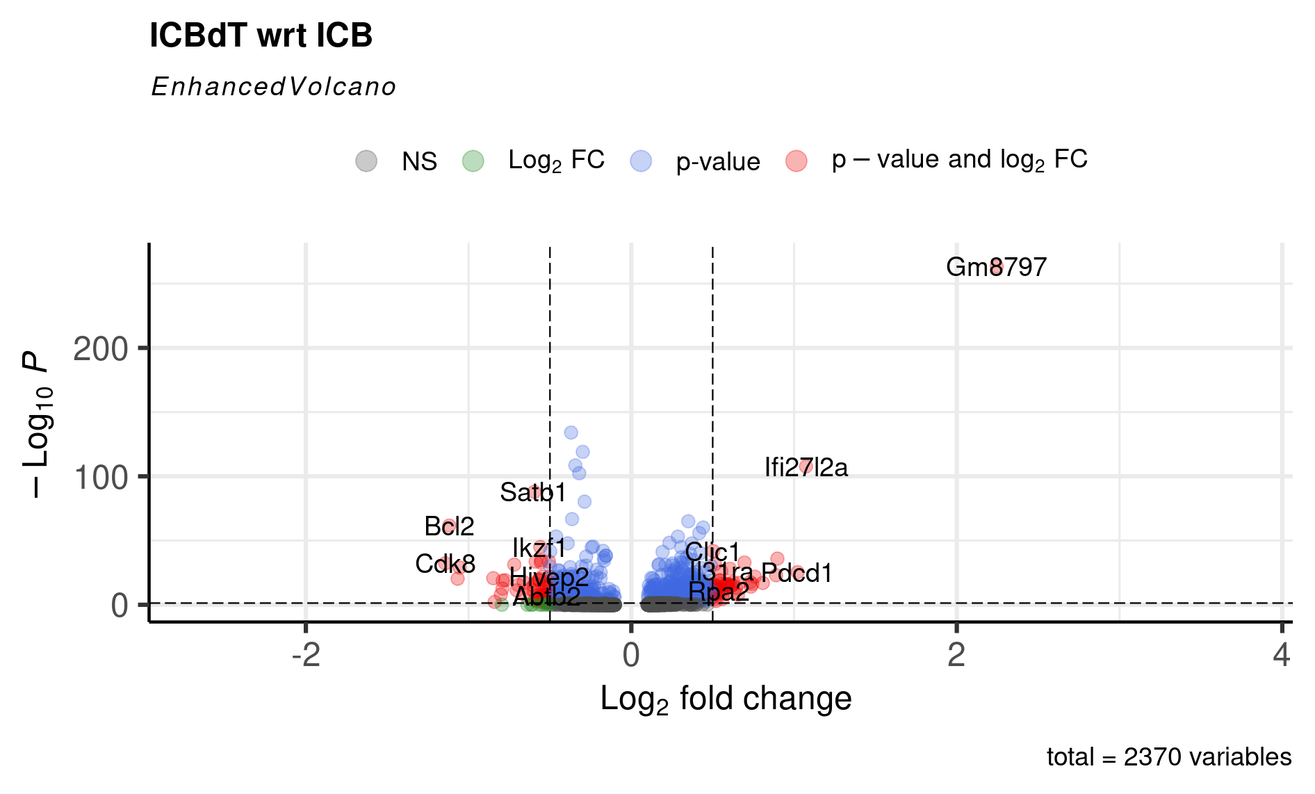
At this point, you can either start doing literature searches for some of these genes and find that for genes like Bcl2, Cdk8, and Znrf3 that were upregulated in ICB CD8 Tcells, the literature suggests- antigen-specific memory CD8 T cells have higher expression of Bcl2 and Cdk8; and Znrf3 has been implicated in CD8 T cells’ anti-tumor response following anti-PD-1 therapy. Also, we replicate the original paper’s findings of ICBdT CD8 T cells upregulating T cell exhaustion markers like Tigit and Pdcd1.
But we can also use gene set and pathway analyses to try and determine what processes the cells may be involved in.
Same as the epithelial cells, let’s create a TSV file containing our DE results for use in pathway analysis by rerunning FindMarkers with the logfc.threshold parameter set to 0.
#rerun FindMarkers
cd8tcells_de_gsea <- FindMarkers(merged_cd8tcells, ident.1 = "ICBdT",
  ident.2 = "ICB", min.pct=0.25, logfc.threshold=0)
#save this table as a TSV file (first move index to first column)
cd8tcells_de_gsea <- tibble::rownames_to_column(cd8tcells_de_gsea, var = "gene")
write.table(x = cd8tcells_de_gsea, file = 'outdir_single_cell_rna/cd8tcells_de_gsea.tsv', sep='\t', row.names = FALSE)
Try using the pseudobulk aggregated expression for the CD8 T cells yourself!
Hint: Aggregate by orig.ident and experimental_condition. (Click here to get the answer)
orig.ident and experimental_condition. (Click here to get the answer)
# Aggregate counts for each sample and cluster combination
pb_cd8tcells <- AggregateExpression(merged_cd8tcells, assays = 'RNA',
                                         return.seurat = T, group.by = c('orig.ident', 'experimental_condition'))

# See the first few rows of the log normalized data layer
print(head(pb_cd8tcells@assays$RNA$data))

# Change ident to seurat clusters
Idents(pb_cd8tcells) <- "experimental_condition"

# Use FindMarkers with DESeq2 as the test to compare cluster 9 wrt cluster 12
pb_cd8tcells_de <- FindMarkers(object = pb_cd8tcells, test.use = "DESeq2",
                                  ident.1 = "ICBdT", ident.2 = "ICB")

# The DESeq2 analysis results in NAs in the pvalue columns for some cases
pb_cd8tcells_de <- na.omit(pb_cd8tcells_de)

# Restrict differentially expressed genes to those with an adjusted p-value less than 0.001
pb_cd8tcells_de_sig <- pb_cd8tcells_de[pb_cd8tcells_de$p_val_adj < 0.01,]

# Compare significantly differentially expressed genes
pb_and_sc_genes <- intersect(rownames(cd8tcells_de_sig), rownames(pb_cd8tcells_de_sig))
only_sc_genes <- setdiff(rownames(cd8tcells_de_sig), rownames(pb_cd8tcells_de_sig))
only_pb_genes <- setdiff(rownames(pb_cd8tcells_de_sig), rownames(cd8tcells_de_sig))

print(paste0("Genes differentially expressed in both single-cell and pseudobulk: ", length(pb_and_sc_genes)))
print(paste0("Genes differentially expressed in single-cell but not pseudobulk: ", length(only_sc_genes)))
print(paste0("Genes differentially expressed in pseudobulk but not single-cell: ", length(only_pb_genes)))
Hmm looks like we barely have any significant DE genes for the pseudobulk data. Let's look at a few of the genes we pulled out earlier:
VlnPlot(merged_cd8tcells, features = c('Bcl2', 'Cdk8', 'Znrf3'), group.by = 'orig.ident')
print(pb_cd8tcells_de[rownames(pb_cd8tcells_de) %in% c('Bcl2', 'Cdk8', 'Znrf3'), ])
It looks like those genes didn't get past the multiple hypothesis correcting. In practice, it would be a judgement call on whether or not you expect these to be 'real' and how you want to validate them.