Differential Splicing

« Transcript Assembly Merge Course Transcript Assembly Visualization »

RNA-seq_Flowchart5

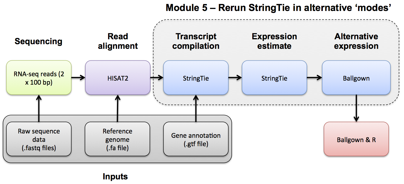
Use Ballgown and Stringtie to compare the UHR and HBR conditions against reference guided and de novo transcript assemblies.

Refer to the Stringtie manual for a more detailed explanation: https://ccb.jhu.edu/software/stringtie/index.shtml?t=manual

The Ballgown github page also has documentation for getting started with ballgown: https://github.com/alyssafrazee/ballgown

Calculate UHR and HBR expression estimates, for known/novel (reference guided mode) transcripts

Re-run Stringtie using the reference guided merged GTF, and output tables for Ballgown. Store the results in a new directory so that we can still examine the results generated without the merged GTF.

cd $RNA_HOME/expression/stringtie/
mkdir ref_guided_merged
cd ref_guided_merged

stringtie --rf -p 4 -G ../ref_guided/stringtie_merged.gtf -e -B -o HBR_Rep1/transcripts.gtf $RNA_ALIGN_DIR/HBR_Rep1.bam
stringtie --rf -p 4 -G ../ref_guided/stringtie_merged.gtf -e -B -o HBR_Rep2/transcripts.gtf $RNA_ALIGN_DIR/HBR_Rep2.bam
stringtie --rf -p 4 -G ../ref_guided/stringtie_merged.gtf -e -B -o HBR_Rep3/transcripts.gtf $RNA_ALIGN_DIR/HBR_Rep3.bam

stringtie --rf -p 4 -G ../ref_guided/stringtie_merged.gtf -e -B -o UHR_Rep1/transcripts.gtf $RNA_ALIGN_DIR/UHR_Rep1.bam
stringtie --rf -p 4 -G ../ref_guided/stringtie_merged.gtf -e -B -o UHR_Rep2/transcripts.gtf $RNA_ALIGN_DIR/UHR_Rep2.bam
stringtie --rf -p 4 -G ../ref_guided/stringtie_merged.gtf -e -B -o UHR_Rep3/transcripts.gtf $RNA_ALIGN_DIR/UHR_Rep3.bam

Run Ballgown using the reference guided, merged transcripts

mkdir -p $RNA_HOME/de/ballgown/ref_guided_merged/
cd $RNA_HOME/de/ballgown/ref_guided_merged/

printf "\"ids\",\"type\",\"path\"\n\"UHR_Rep1\",\"UHR\",\"$RNA_HOME/expression/stringtie/ref_guided_merged/UHR_Rep1\"\n\"UHR_Rep2\",\"UHR\",\"$RNA_HOME/expression/stringtie/ref_guided_merged/UHR_Rep2\"\n\"UHR_Rep3\",\"UHR\",\"$RNA_HOME/expression/stringtie/ref_guided_merged/UHR_Rep3\"\n\"HBR_Rep1\",\"HBR\",\"$RNA_HOME/expression/stringtie/ref_guided_merged/HBR_Rep1\"\n\"HBR_Rep2\",\"HBR\",\"$RNA_HOME/expression/stringtie/ref_guided_merged/HBR_Rep2\"\n\"HBR_Rep3\",\"HBR\",\"$RNA_HOME/expression/stringtie/ref_guided_merged/HBR_Rep3\"\n" > UHR_vs_HBR.csv

Please see Differential Expression for details on running ballgown to determine a DE gene/transcript list.

Calculate UHR and HBR expression estimates, for known/novel (de novo mode) transcripts:

Re-run Stringtie using the de novo merged GTF, and output tables for Ballgown. Store the results in a new directory so that we can still examine the results generated without the merged GTF.

cd $RNA_HOME/expression/stringtie/de_novo
cd $RNA_HOME/expression/stringtie/
mkdir de_novo_merged
cd de_novo_merged

stringtie --rf -p 4 -G ../de_novo/stringtie_merged.gtf -e -B -o HBR_Rep1/transcripts.gtf $RNA_ALIGN_DIR/HBR_Rep1.bam
stringtie --rf -p 4 -G ../de_novo/stringtie_merged.gtf -e -B -o HBR_Rep2/transcripts.gtf $RNA_ALIGN_DIR/HBR_Rep2.bam
stringtie --rf -p 4 -G ../de_novo/stringtie_merged.gtf -e -B -o HBR_Rep3/transcripts.gtf $RNA_ALIGN_DIR/HBR_Rep3.bam

stringtie --rf -p 4 -G ../de_novo/stringtie_merged.gtf -e -B -o UHR_Rep1/transcripts.gtf $RNA_ALIGN_DIR/UHR_Rep1.bam
stringtie --rf -p 4 -G ../de_novo/stringtie_merged.gtf -e -B -o UHR_Rep2/transcripts.gtf $RNA_ALIGN_DIR/UHR_Rep2.bam
stringtie --rf -p 4 -G ../de_novo/stringtie_merged.gtf -e -B -o UHR_Rep3/transcripts.gtf $RNA_ALIGN_DIR/UHR_Rep3.bam

Run Ballgown using the de novo, merged transcripts

mkdir -p $RNA_HOME/de/ballgown/de_novo_merged/
cd $RNA_HOME/de/ballgown/de_novo_merged/

printf "\"ids\",\"type\",\"path\"\n\"UHR_Rep1\",\"UHR\",\"$RNA_HOME/expression/stringtie/de_novo_merged/UHR_Rep1\"\n\"UHR_Rep2\",\"UHR\",\"$RNA_HOME/expression/stringtie/de_novo_merged/UHR_Rep2\"\n\"UHR_Rep3\",\"UHR\",\"$RNA_HOME/expression/stringtie/de_novo_merged/UHR_Rep3\"\n\"HBR_Rep1\",\"HBR\",\"$RNA_HOME/expression/stringtie/de_novo_merged/HBR_Rep1\"\n\"HBR_Rep2\",\"HBR\",\"$RNA_HOME/expression/stringtie/de_novo_merged/HBR_Rep2\"\n\"HBR_Rep3\",\"HBR\",\"$RNA_HOME/expression/stringtie/de_novo_merged/HBR_Rep3\"\n" > UHR_vs_HBR.csv

Please see Differential Expression for details on running ballgown to determine a DE gene/transcript list.

« Transcript Assembly Merge Course Transcript Assembly Visualization »

Transcript Assembly Merge

« De Novo Transcript Assembly Course Differential Splicing »

RNA-seq_Flowchart5

Stringtie Merge

Use Stringtie to merge predicted transcripts from all libraries into a unified transcriptome. Refer to the Stringtie manual for a more detailed explanation:

https://ccb.jhu.edu/software/stringtie/index.shtml?t=manual

Options specified below:

assembly_GTF_list.txt is a text file “manifest” with a list (one per line) of GTF files that you would like to merge together into a single GTF file.
–rf tells StringTie that our data is stranded and to use the correct strand specific mode (i.e. assume a stranded library fr-firststrand).
-p 4 tells stringtie to use eight CPUs
-o tells stringtie to write output to a particular file or directory
-G tells stringtie where to find reference gene annotations. It will use these annotations to gracefully merge novel isoforms (for de novo runs) and known isoforms and maximize overall assembly quality.

Merge all 6 Stringtie results so that they will have the same set of transcripts for comparison purposes:

For reference guided mode:

cd $RNA_HOME/expression/stringtie/ref_guided/
ls -1 *Rep*/transcripts.gtf > assembly_GTF_list.txt
cat assembly_GTF_list.txt
stringtie --rf --merge -p 4 -o stringtie_merged.gtf -G $RNA_REF_GTF assembly_GTF_list.txt

What do the resulting transcripts look like?

awk '{if($3=="transcript") print}' stringtie_merged.gtf | cut -f 1,4,9 | less

Press q to exit the less viewer

Compare reference guided transcripts to the known annotations. This allows us to assess the quality of transcript predictions made from assembling the RNA-seq data. For more details, refer to the Stringtie GFF Utilities and Cuffcompare manuals.

gffcompare -r $RNA_REF_GTF -o gffcompare stringtie_merged.gtf
cat gffcompare.stats

What does the merged annotation look like after comparing it to known annotation? How are the GTF lines different?

awk '{if($3=="transcript") print}' gffcompare.annotated.gtf | cut -f 1,4,9 | less

Press ‘q’ to exit the less viewer

For de novo mode (again, we do not provide an Ensembl GTF):

cd $RNA_HOME/expression/stringtie/de_novo/
ls -1 *Rep*/transcripts.gtf > assembly_GTF_list.txt
cat assembly_GTF_list.txt
stringtie --rf --merge -p 4 -o stringtie_merged.gtf assembly_GTF_list.txt

Compare the de novo merged transcripts to the known annotations:

gffcompare -r $RNA_REF_GTF -o gffcompare stringtie_merged.gtf
cat gffcompare.stats