Posts
My thoughts and ideas
Welcome to the blog
My thoughts and ideas
Introduction to bioinformatics for RNA sequence analysis
Annotating cells in single-cell gene expression data is an active area of research. Defining a cell type can be challenging because of two fundamental reasons. One, gene expression levels are not discrete and mostly on a continuum; and two, differences in gene expression do not always translate to differences in cellular function (Pasquini et al.). The field is growing and rapidly changing due to the advent of different kinds of annotation tools, and the creation of multiple scRNA-seq databases (Wang et al.).
One way to assign cell type annotation is through web resources. They are relatively easy to use and do not require advanced level scripting or programming skills. Examples include Azimuth, Tabula Sapiens, and SciBet. Researchers sometimes try both methods with multiple tools when performing the cell type annotation. In addition, it is also recommended to validate your annotation by experiments, statistical analysis, or consulting subject matter experts.
Methods for assigning cell types usually fall into one of two categories:
Databases with marker genes for manual annotation: These databases contain marker genes for various cell types (mostly human and mouse). Using the marker genes in these databases, you can annotate the cells in your datasets. For example, if you are using 10x Genomics Loupe Browser, you will be able to find top differentially expressed genes for each cluster. You can then search the genes in the database to find out if they are marker genes for specific cell types. You may need to search multiple top genes in each cluster to be sure about the cell type. Depending on the complexity of the dataset and prior knowledge on the cell types, this process could be laborious and time-consuming.
Resources for automated cell type annotation (reference-based): There are tools developed by the community for automatically annotating cells by comparing new data with existing references. In this article, we will highlight a few web tools that do not require any programming skills. A major limitation of these tools is that the quality of the results heavily depends on the quality of the pre-annotated reference datasets.
First, we need to load the relevant libraries.
library(SingleR)
library(celldex)
library(Seurat)
library(cowplot)

merged <- readRDS("outdir_single_cell_rna/rep135_clustered.rds")
Alternatively, we can download a copy of this rds object and then load it in.
url <- "https://genomedata.org/cri-workshop/rep135_clustered.rds"
file_name <- "rep135_clustered.rds"
file_path <- "outdir_single_cell_rna/"
download.file(url, paste(file_path, file_name, sep = ""), mode = "wb")
merged <- readRDS('outdir_single_cell_rna/rep135_clustered.rds')
The following function provides normalized expression values of 830 microarray samples generated by ImmGen from pure populations of murine immune cells. The samples were processed and normalized as described in Aran, Looney and Liu et al. (2019), i.e., CEL files from the Gene Expression Omnibus (GEO; GSE15907 and GSE37448), were downloaded, processed, and normalized using the robust multi-array average (RMA) procedure on probe-level data. This dataset consists of 20 broad cell types (“label.main”) and 253 finely resolved cell subtypes (“label.fine”). The subtypes have also been mapped to the Cell Ontology (“label.ont”, if cell.ont is not “none”), which can be used for further programmatic queries.
#cell typing with single R
#load singleR immgen reference
ref_immgen <- celldex::ImmGenData()
Calling the ImmGenData() function returns a SummarizedExperiment object containing a matrix of log-expression values with sample-level labels.
ref_immgen
#result of calling the above ref_immgen function
class: SummarizedExperiment
dim: 22134 830
metadata(0):
assays(1): logcounts
rownames(22134): Zglp1 Vmn2r65 ... Tiparp Kdm1a
rowData names(0):
colnames(830):
  GSM1136119_EA07068_260297_MOGENE-1_0-ST-V1_MF.11C-11B+.LU_1.CEL
  GSM1136120_EA07068_260298_MOGENE-1_0-ST-V1_MF.11C-11B+.LU_2.CEL
  ...
  GSM920654_EA07068_201214_MOGENE-1_0-ST-V1_TGD.VG4+24ALO.E17.TH_1.CEL
  GSM920655_EA07068_201215_MOGENE-1_0-ST-V1_TGD.VG4+24ALO.E17.TH_2.CEL
colData names(3): label.main label.fine label.ont
Now let’s see what each of the labels look like:
head(ref_immgen$label.main, n=10)
From the main labels, we can see that we get general cell types such as Macrophages and Monocytes.
[1] "Macrophages" "Macrophages" "Macrophages"
[4] "Macrophages" "Macrophages" "Macrophages"
[7] "Monocytes"   "Monocytes"   "Monocytes"
[10] "Monocytes"
head(ref_immgen$label.fine, n=10)
From the fine labels, we can see that we start to subtype the more general cell types we saw above. So rather than seeing 6 labels for Macrophages we now see specific Macrophage types such as Macrophages (MF.11C-11B+).
[1] "Macrophages (MF.11C-11B+)" "Macrophages (MF.11C-11B+)"
[3] "Macrophages (MF.11C-11B+)" "Macrophages (MF.ALV)"
[5] "Macrophages (MF.ALV)"      "Macrophages (MF.ALV)"
[7] "Monocytes (MO.6+I-)"       "Monocytes (MO.6+2+)"
[9] "Monocytes (MO.6+2+)"       "Monocytes (MO.6+2+)"
head(ref_immgen$label.ont, n=10)
From the ont labels, we can see that we start to subtypes are now mapped to Cell Ontology IDs.
[1] "CL:0000235" "CL:0000235" "CL:0000235" "CL:0000583" "CL:0000583"
[6] "CL:0000583" "CL:0000576" "CL:0000576" "CL:0000576" "CL:0000576"
#generate predictions for our seurat object
predictions_main = SingleR(test = GetAssayData(merged),
                      ref = ref_immgen,
                      labels = ref_immgen$label.main)

predictions_fine = SingleR(test = GetAssayData(merged),
                           ref = ref_immgen,
                           labels = ref_immgen$label.fine)
What do these objects look like?
head(predictions_main)
You should see something like the below, where each row is a barcode with columns for scores, labels (assigned cell type), delta, and pruned.labels.
DataFrame with 6 rows and 4 columns
                                                         scores
                                                       <matrix>
Rep1_ICBdT_AAACCTGAGCCAACAG-1 0.4156037:0.4067582:0.2845856:...
Rep1_ICBdT_AAACCTGAGCCTTGAT-1 0.4551058:0.3195934:0.2282272:...
Rep1_ICBdT_AAACCTGAGTACCGGA-1 0.0717647:0.0621878:0.0710026:...
Rep1_ICBdT_AAACCTGCACGGCCAT-1 0.2774994:0.2569566:0.2483387:...
Rep1_ICBdT_AAACCTGCACGGTAAG-1 0.3486259:0.3135662:0.3145100:...
Rep1_ICBdT_AAACCTGCATGCCACG-1 0.0399733:0.0229926:0.0669236:...
                                   labels delta.next
                              <character>  <numeric>
Rep1_ICBdT_AAACCTGAGCCAACAG-1         NKT  0.0124615
Rep1_ICBdT_AAACCTGAGCCTTGAT-1     B cells  0.1355124
Rep1_ICBdT_AAACCTGAGTACCGGA-1 Fibroblasts  0.1981683
Rep1_ICBdT_AAACCTGCACGGCCAT-1    NK cells  0.0577608
Rep1_ICBdT_AAACCTGCACGGTAAG-1     T cells  0.1038542
Rep1_ICBdT_AAACCTGCATGCCACG-1 Fibroblasts  0.2443470
                              pruned.labels
                                <character>
Rep1_ICBdT_AAACCTGAGCCAACAG-1           NKT
Rep1_ICBdT_AAACCTGAGCCTTGAT-1       B cells
Rep1_ICBdT_AAACCTGAGTACCGGA-1   Fibroblasts
Rep1_ICBdT_AAACCTGCACGGCCAT-1      NK cells
Rep1_ICBdT_AAACCTGCACGGTAAG-1       T cells
Rep1_ICBdT_AAACCTGCATGCCACG-1   Fibroblasts
Okay…but what do these columns actually tell us?
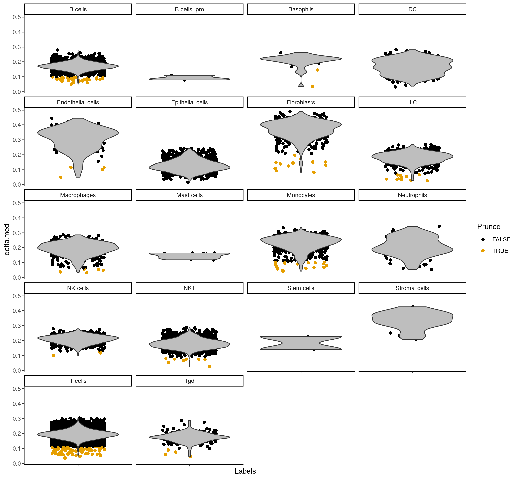
The scores column contains a matrix for each barcode that corresponds to how confident SingleR is in assigning each cell type to the barcode for that row. The labels column is the most confident assignment singleR has for that particular barcode. The delta column contains the “delta” value for each cell, which is the gap, or the difference between the score for the assigned label and the median score across all labels. If the delta is small, this indicates that the cell matches all labels with the same confidence, so the assigned label is not very meaningful. SingleR can discard cells with low delta values caused by (i) ambiguous assignments with closely related reference labels and (ii) incorrect assignments that match poorly to all reference labels – so in the pruned.labels column you will find “cleaner” or more reliable labels.
How many cells have low confidence labels?
unique(predictions_main$pruned.labels)
 [1] "NKT"               "B cells"
 [3] "Fibroblasts"       "NK cells"
 [5] "T cells"           "Neutrophils"
 [7] "DC"                "Monocytes"
 [9] "ILC"               "Epithelial cells"
[11] "Macrophages"       "Basophils"
[13] "Tgd"               "Mast cells"
[15] "Endothelial cells" NA
[17] "Stem cells"        "Stromal cells"
[19] "B cells, pro"
table(predictions_main$pruned.labels)
          B cells      B cells, pro         Basophils
             3219                 3                33
               DC Endothelial cells  Epithelial cells
              295                67              1238
      Fibroblasts               ILC       Macrophages
              577               752               454
       Mast cells         Monocytes       Neutrophils
               11               617                92
         NK cells               NKT        Stem cells
              562              2241                 2
    Stromal cells           T cells               Tgd
               18             12631               189
table(predictions_main$labels)
          B cells      B cells, pro         Basophils
             3253                 3                37
               DC Endothelial cells  Epithelial cells
              295                71              1238
      Fibroblasts               ILC       Macrophages
              589               763               459
       Mast cells         Monocytes       Neutrophils
               11               633                92
         NK cells               NKT        Stem cells
              565              2249                 2
    Stromal cells           T cells               Tgd
               18             12714               193
summary(is.na(predictions_main$pruned.labels))
   Mode   FALSE    TRUE
logical   23001     184
Are there more or less pruned labels for the fine labels?
summary(is.na(predictions_fine$pruned.labels))
   Mode   FALSE    TRUE
logical   23006     179
Now that we understand what the singleR dataframe looks like and what the data contains, let’s begin to visualize the data.
plotDeltaDistribution(predictions_main, ncol = 4, dots.on.top = FALSE)
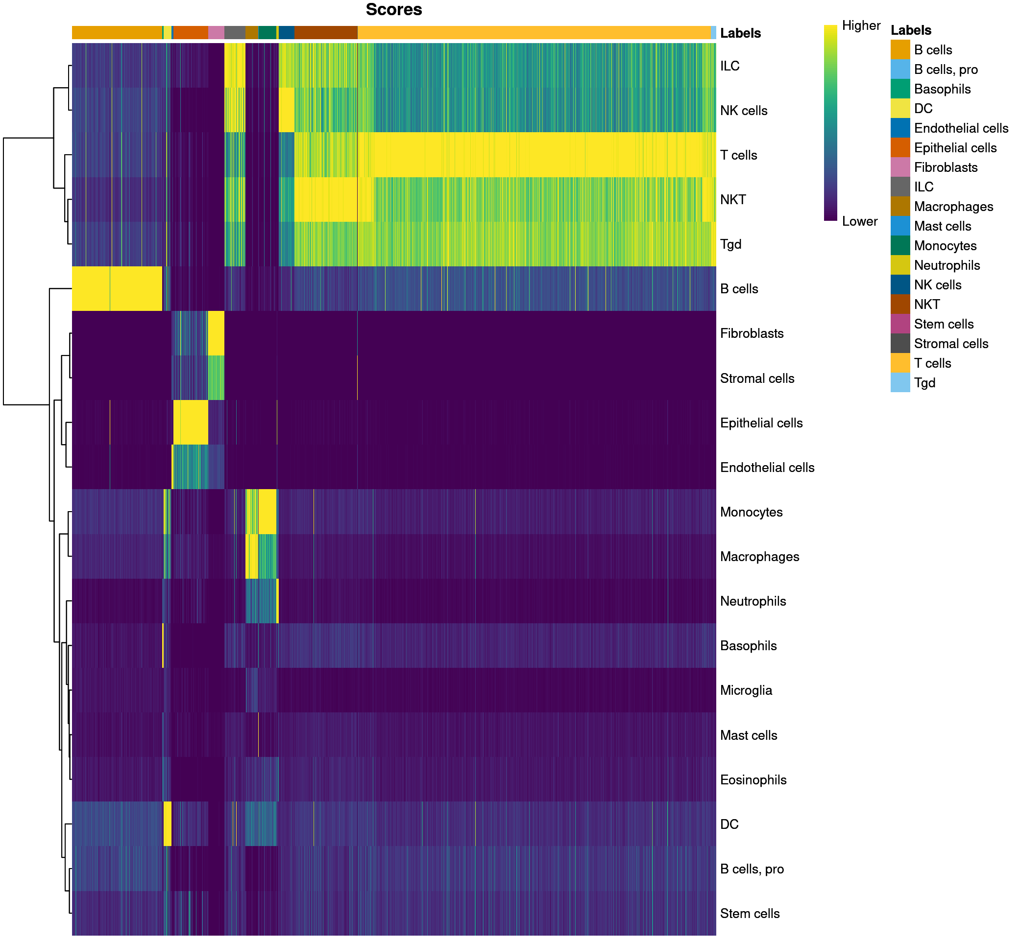
plotScoreHeatmap(predictions_main)
Rather than only working with the singleR dataframe, we can add the labels to our Seurat data object as a metadata field, so let’s add the cell type labels to our seurat object.
#add main labels to object
merged[['immgen_singler_main']] = rep('NA', ncol(merged))
merged$immgen_singler_main[rownames(predictions_main)] = predictions_main$labels

#add fine labels to object
merged[['immgen_singler_fine']] = rep('NA', ncol(merged))
merged$immgen_singler_fine[rownames(predictions_fine)] = predictions_fine$labels
How do our samples differ in their relative cell composition?
#visualizing the relative proportion of cell types across our samples
library(viridis)
library(ggplot2)
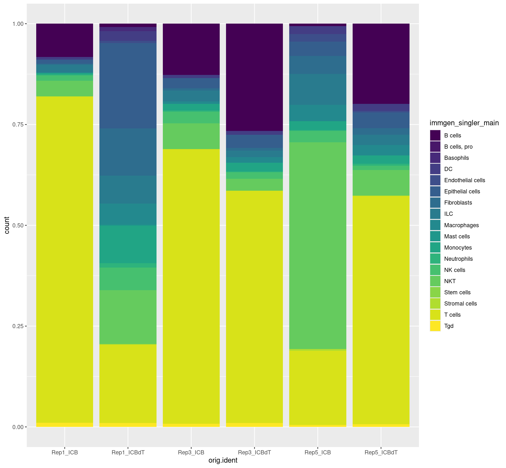
ggplot(merged[[]], aes(x = orig.ident, fill = immgen_singler_main)) + geom_bar(position = "fill") + scale_fill_viridis(discrete = TRUE)
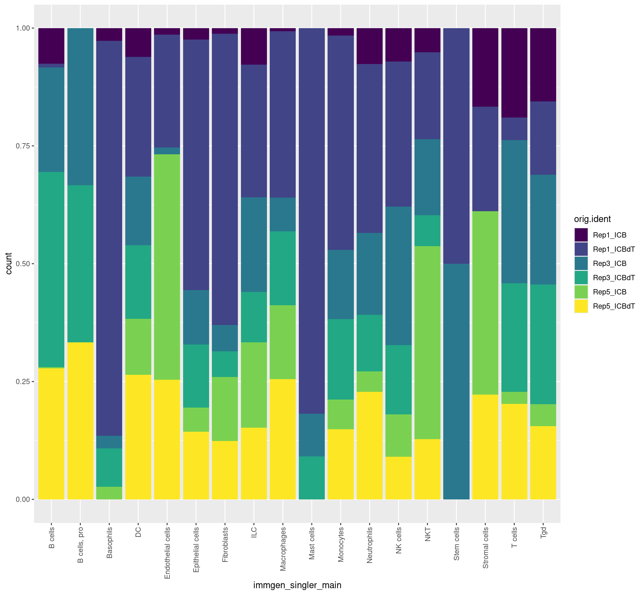
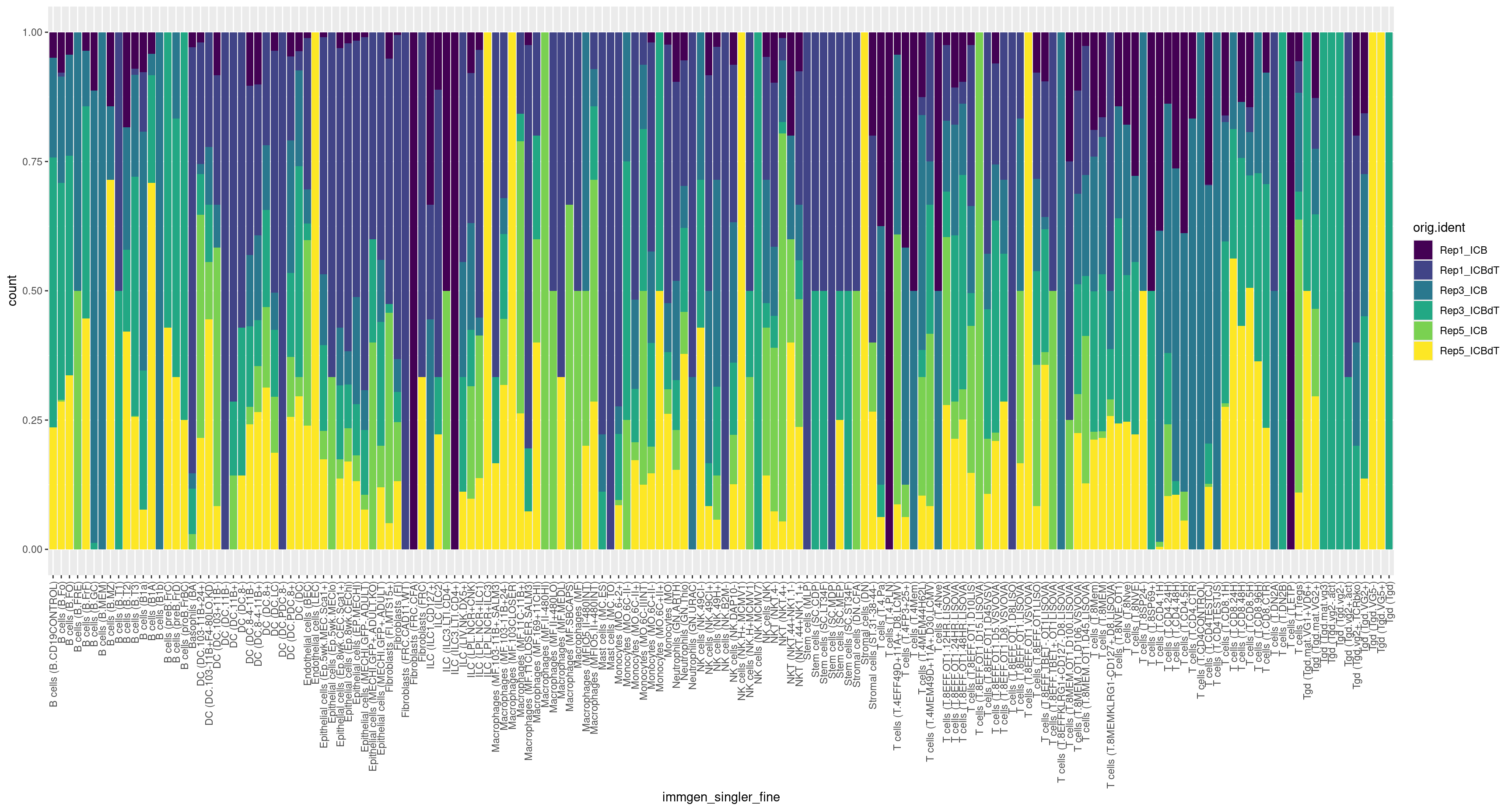
We can also flip the samples and cell labels and view this data as below.
ggplot(merged[[]], aes(x = immgen_singler_main, fill = orig.ident)) + geom_bar(position = "fill") + theme(axis.text.x = element_text(angle = 90, vjust = 0.5, hjust=1)) + scale_fill_viridis(discrete = TRUE)

ggplot(merged[[]], aes(x = immgen_singler_fine, fill = orig.ident)) + geom_bar(position = "fill") + theme(axis.text.x = element_text(angle = 90, vjust = 0.5, hjust=1)) + scale_fill_viridis(discrete = TRUE)
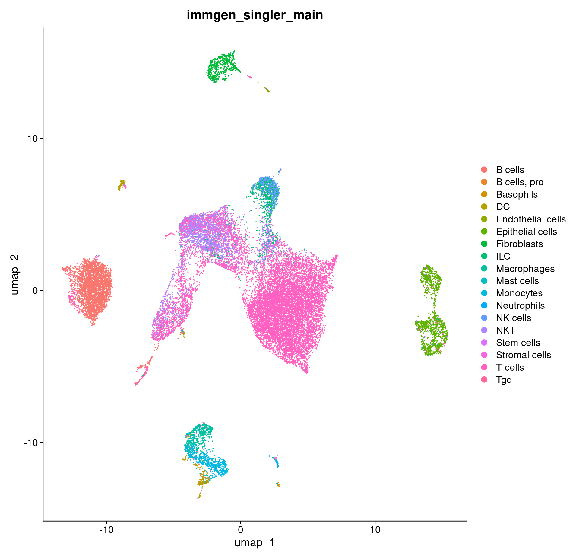
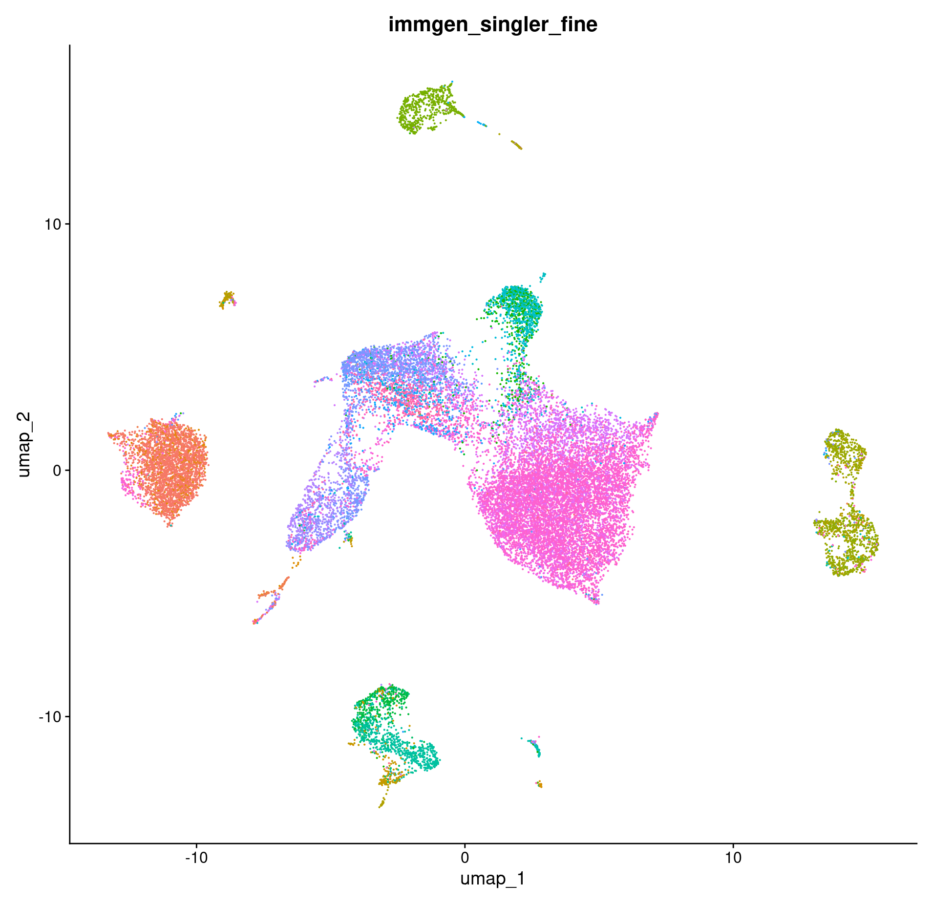
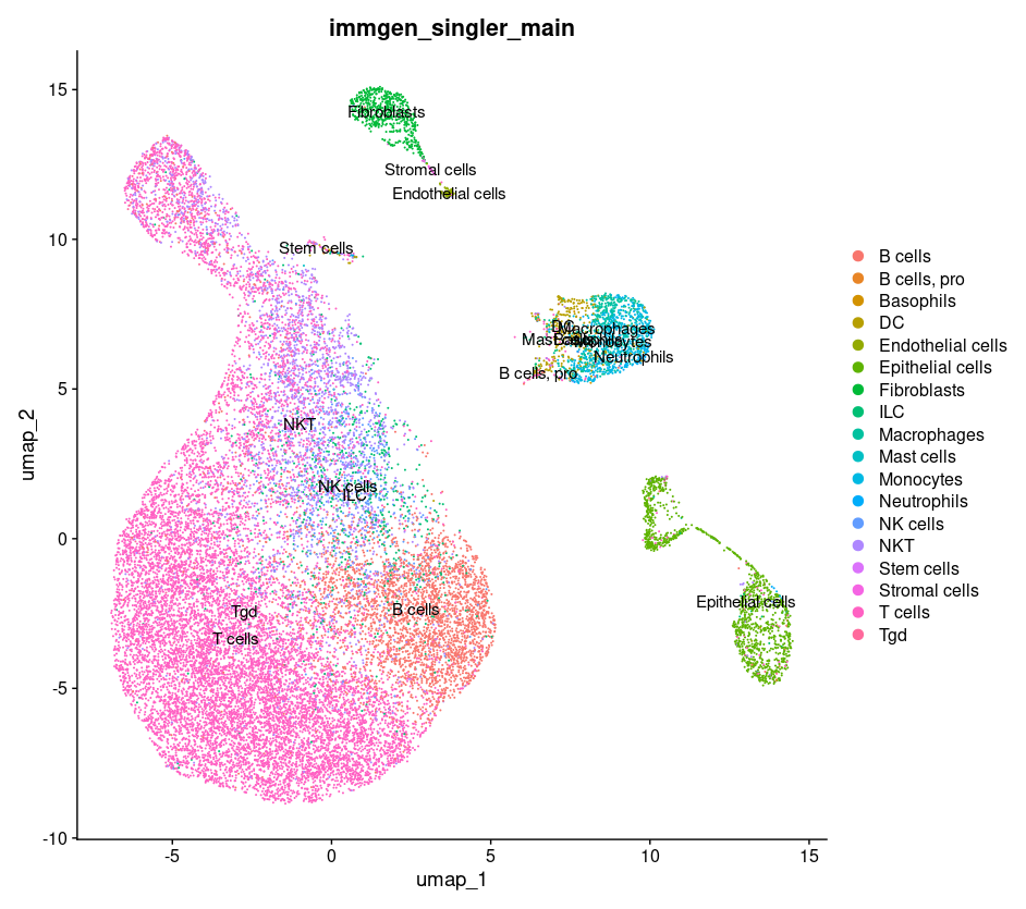
How do our cell type annotations map to our clusters we defined previously?
#plotting cell types on our umaps
DimPlot(merged, group.by = c("immgen_singler_main"))

DimPlot(merged, group.by = c("immgen_singler_fine")) + NoLegend()
We previously used the ImmGen dataset but what if we wanted to use a different one?
celldex::listReferences()
[1] "blueprint_encode"
[2] "dice"
[3] "hpca"
[4] "immgen"
[5] "monaco_immune"
[6] "mouse_rnaseq"
[7] "novershtern_hematopoietic"
Let’s try using the mouse_rnaseq one and see how our labels differ.
This dataset was contributed by the Benayoun Lab that identified, downloaded and processed data sets on GEO that corresponded to sorted cell types Benayoun et al., 2019.
The dataset contains 358 mouse RNA-seq samples annotated to 18 main cell types (“label.main”). These are split further into 28 subtypes (“label.fine”). The subtypes have also been mapped to the Cell Ontology as with the ImmGen reference.
ref_mouserna <- celldex::MouseRNAseqData()
If we look at this reference, we can see that it also has the main, fine, and ont labels that we saw with the ImmGen reference.
ref_mouserna
class: SummarizedExperiment
dim: 21214 358
metadata(0):
assays(1): logcounts
rownames(21214): Xkr4 Rp1 ... LOC100039574 LOC100039753
rowData names(0):
colnames(358): ERR525589Aligned ERR525592Aligned ... SRR1044043Aligned
  SRR1044044Aligned
colData names(3): label.main label.fine label.ont
predictions_mouse_main = SingleR(test = GetAssayData(merged),
                      ref = ref_mouserna,
                      labels = ref_mouserna$label.main)

predictions_mouse_fine = SingleR(test = GetAssayData(merged),
                           ref = ref_mouserna,
                           labels = ref_mouserna$label.fine)
merged[['mouserna_singler_main']] = rep('NA', ncol(merged))
merged$mouserna_singler_main[rownames(predictions_mouse_main)] = predictions_mouse_main$labels

#add fine labels to object
merged[['mouserna_singler_fine']] = rep('NA', ncol(merged))
merged$mouserna_singler_fine[rownames(predictions_mouse_fine)] = predictions_mouse_fine$labels
Let’s visualize how the labeling of our cells differs between the main labels from ImmGen and MouseRNA.
table(predictions_main$labels)
table(predictions_mouse_main$labels)
          B cells      B cells, pro         Basophils                DC Endothelial cells
             3253                 3                37               295                71
 Epithelial cells       Fibroblasts               ILC       Macrophages        Mast cells
             1238               589               763               459                11
        Monocytes       Neutrophils          NK cells               NKT        Stem cells
              633                92               565              2249                 2
    Stromal cells           T cells               Tgd
               18             12714               193


       Adipocytes           B cells   Dendritic cells Endothelial cells       Fibroblasts
                4              3325                94               245               979
     Granulocytes       Hepatocytes       Macrophages         Monocytes          NK cells
              116               652               185              1013              1341
          T cells
            15231
p1 <- DimPlot(merged, group.by = c("immgen_singler_main")) + scale_colour_viridis(option = 'turbo', discrete = TRUE)
p2 <- DimPlot(merged, group.by = c("mouserna_singler_main")) + scale_colour_viridis(option = 'turbo', discrete = TRUE)
p <- plot_grid(p1, p2, ncol = 2)
p
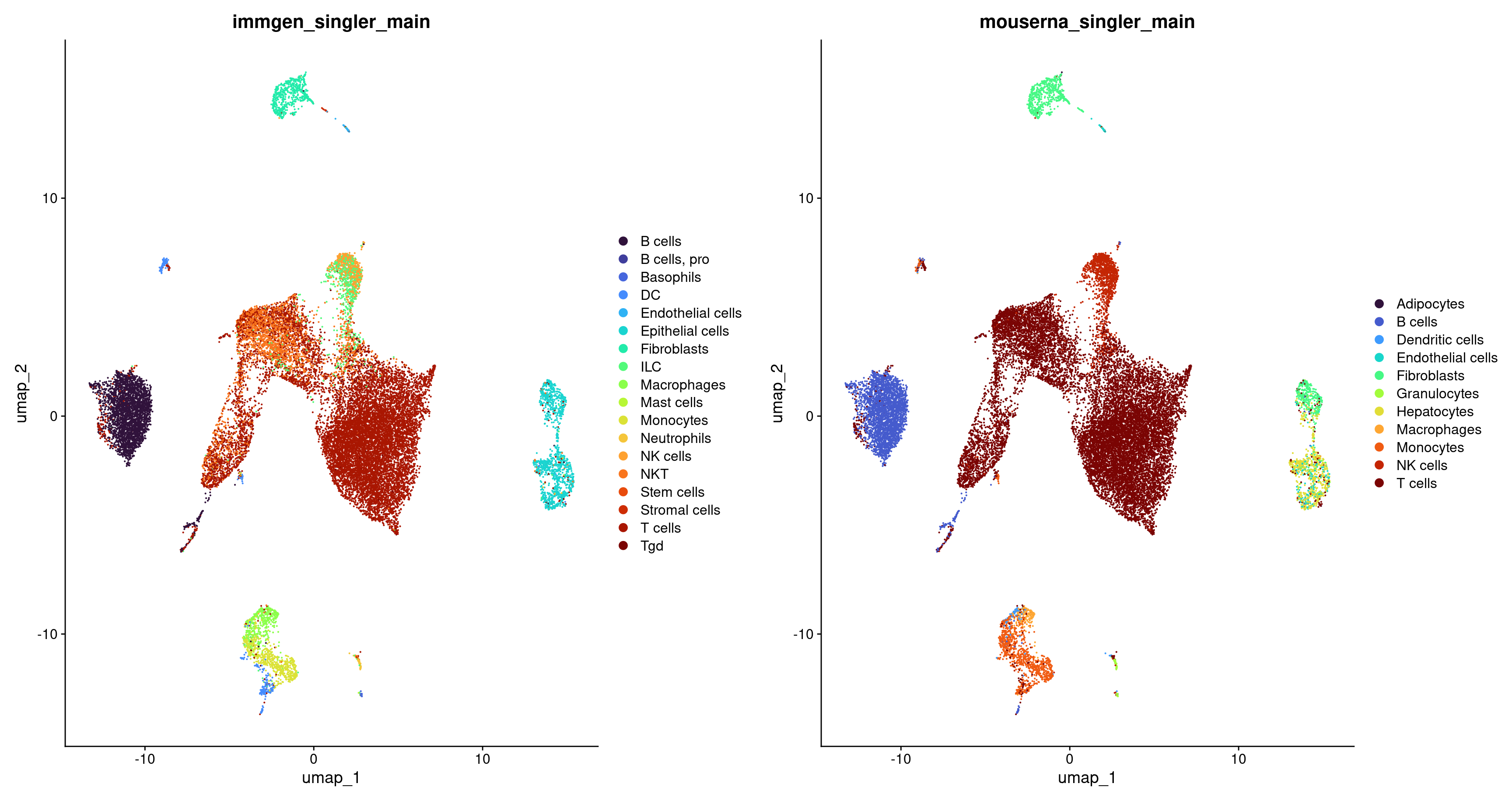
As one might expect, the choice of reference can have a major impact on the annotation results. It’s essential to choose a reference dataset encompassing a broader spectrum of labels than those expected in our test dataset. Trust in the appropriateness of labels assigned by the original authors to reference samples is often a leap of faith, and it’s unsurprising that certain references outperform others due to differences in sample preparation quality. Ideally, we favor a reference generated using a technology or protocol similar to our test dataset, although this consideration is typically not an issue when using SingleR() for annotating well-defined cell types.
Users are advised to read the relevant vignette for more details about the available references as well as some recommendations on which to use. (As an aside, the ImmGen dataset and other references were originally supplied along with SingleR itself but have since been migrated to the separate celldex package for more general use throughout Bioconductor.) Of course, as we shall see in the next Chapter, it is entirely possible to supply your own reference datasets instead; all we need are log-expression values and a set of labels for the cells or samples
We know that the UMAP shape changes when we use different numbers of PCs but why does the UMAP shape change? Lets try creating a UMAP with only 5 PCs.
merged_5PC <- RunUMAP(merged, dims = 1:5)

DimPlot(merged_5PC, label = TRUE, group.by = 'immgen_singler_main')

DimHeatmap(merged, dims = 1:5, balanced = TRUE, cells = 500)
We see that the cells form much more general clusters. For example, the immune cells are just in one big blob. When we increase our PCs we increase the amount of information that can be used to tease apart more specfic cell types. The distinct B cell cluster we saw earlier was only possible because we provided enough genetic expression information in the PCs we chose.
Let’s save our seurat objects to use in future sections.
saveRDS(merged, file = "outdir_single_cell_rna/preprocessed_object.rds")