TCR/BCR Repertoire Analysis
In this module, we will use our scRNA seurat object to explore immune receptor T and B cell diversity. To recognize both antigens and tumor neoantigens, T cells generate diverse receptor sequences through somatic V(D)J recombination. B cells perform V(D)J recombination during developement and then, after antigen encounter, use somatic hypermutation to further diversify their receptors.
We will be using scRepertoire to explore TCR and BCR data. This R package provides several convenient processing and visualization functions that are easy to understand and use. We will then add the clonal information for both B and T cells back onto our Seurat object to be used in further analysis.
#BiocManager::install("scRepertoire")

library("scRepertoire")
library("dplyr")
library("Seurat")
Understanding our TCR data
In the output from 10x Genomics Cell Ranger vdj pipeline, the main file that we use to explore our TCR/BCR repertoire is filtered_contig_annotations.csv. filtered_contig_annotations.csv provides high-level annotations of each high-confidence contig from cell-associated barcodes. Each contig aims to represent the complete variable region (and often part of the constant region) of a single TCR or BCR chain from a single cell.
More about the outputs…
Lets read in a filtered contigs file and explore what this file contains. This files contains columns such as high confidence, full length, and productive denoting how likely a contig is a true TCR region. Let’s look at one contig.
setwd("/cloud/project/")
Rep1_ICB_t <- read.csv("data/single_cell_rna/clonotypes_t_posit/Rep1_ICB-t-filtered_contig_annotations.csv")

colnames(Rep1_ICB_t)
head(Rep1_ICB_t, 1)
If we look at one cell barcode, we expect to see see 2 contigs: an alpha chain and a beta chain.
Rep1_ICB_t[Rep1_ICB_t$barcode == "AAACCTGAGCGGATCA-1", 1:10]
             barcode is_cell                   contig_id high_confidence length chain  v_gene d_gene  j_gene c_gene
1 AAACCTGAGCGGATCA-1    true AAACCTGAGCGGATCA-1_contig_1            true    552   TRA TRAV3-3         TRAJ37   TRAC
2 AAACCTGAGCGGATCA-1    true AAACCTGAGCGGATCA-1_contig_2            true    514   TRB  TRBV14  TRBD1 TRBJ1-1  TRBC1
But sometimes we see more than two. You may observe two alpha chains and one beta chain or vice versa. In theory, it is possible for a cell to express two alpha chains and two beta chains, although normally one allele is supressed/expressed for each. What are other explanations for seeing multiple alpha/beta chains assigned to a single cell?
Rep1_ICB_t[Rep1_ICB_t$barcode == "AAACCTGTCAGTCCCT-1", 1:10]
              barcode is_cell                   contig_id high_confidence length chain        v_gene d_gene  j_gene c_gene
8  AAACCTGTCAGTCCCT-1    true AAACCTGTCAGTCCCT-1_contig_1            true    552   TRB        TRBV16  TRBD1 TRBJ1-4  TRBC1
9  AAACCTGTCAGTCCCT-1    true AAACCTGTCAGTCCCT-1_contig_2            true    603   TRA TRAV14D-3-DV8         TRAJ22   TRAC
10 AAACCTGTCAGTCCCT-1    true AAACCTGTCAGTCCCT-1_contig_3            true    558   TRA       TRAV4-3         TRAJ34   TRAC
Take a look at some more barcodes. How often to we have a barcode that just has an alpha and beta chain? How often do we see barcodes with 3+ chains? You can summarize this with the following command.
table(table(Rep1_ICB_t[, "barcode"]))
The column raw_clonotype_id contains clonotype IDs which represent TCRs. There should be only one unique clonotype ID per cell.
Rep1_ICB_t[Rep1_ICB_t$barcode == "AAACCTGTCAGTCCCT-1", "raw_clonotype_id"]
[1] "clonotype1609" "clonotype1609" "clonotype1609"
Using this column we can count the unique cells per clonotype. This would show us if there was expansion of a single TCR (an possible immune response). First we have to get our data into the correct format. We want to count how many times we see raw_clonotype_id, accounting for the fact that there are duplicate barcodes depending on how many chains are making up the clonotype.
Rep1_ICB_clonotype_counts <- Rep1_ICB_t %>%
  distinct(barcode, raw_clonotype_id) %>%  # First get unique barcode-clonotype pairs
  group_by(raw_clonotype_id) %>%
  summarize(cell_count = n()) %>%
  arrange(desc(cell_count))  # Sort by count for better visualization

head(Rep1_ICB_clonotype_counts)
# A tibble: 6 × 2
  raw_clonotype_id cell_count
  <chr>                 <int>
1 clonotype1                8
2 clonotype2                7
3 clonotype3                7
4 clonotype4                5
5 clonotype5                5
6 clonotype6                5
Cellranger will always assign clonotype1 to the clonotype with the most expansion – the greatest number of cells with that TCR. 8 cells is not a lot of expansion…
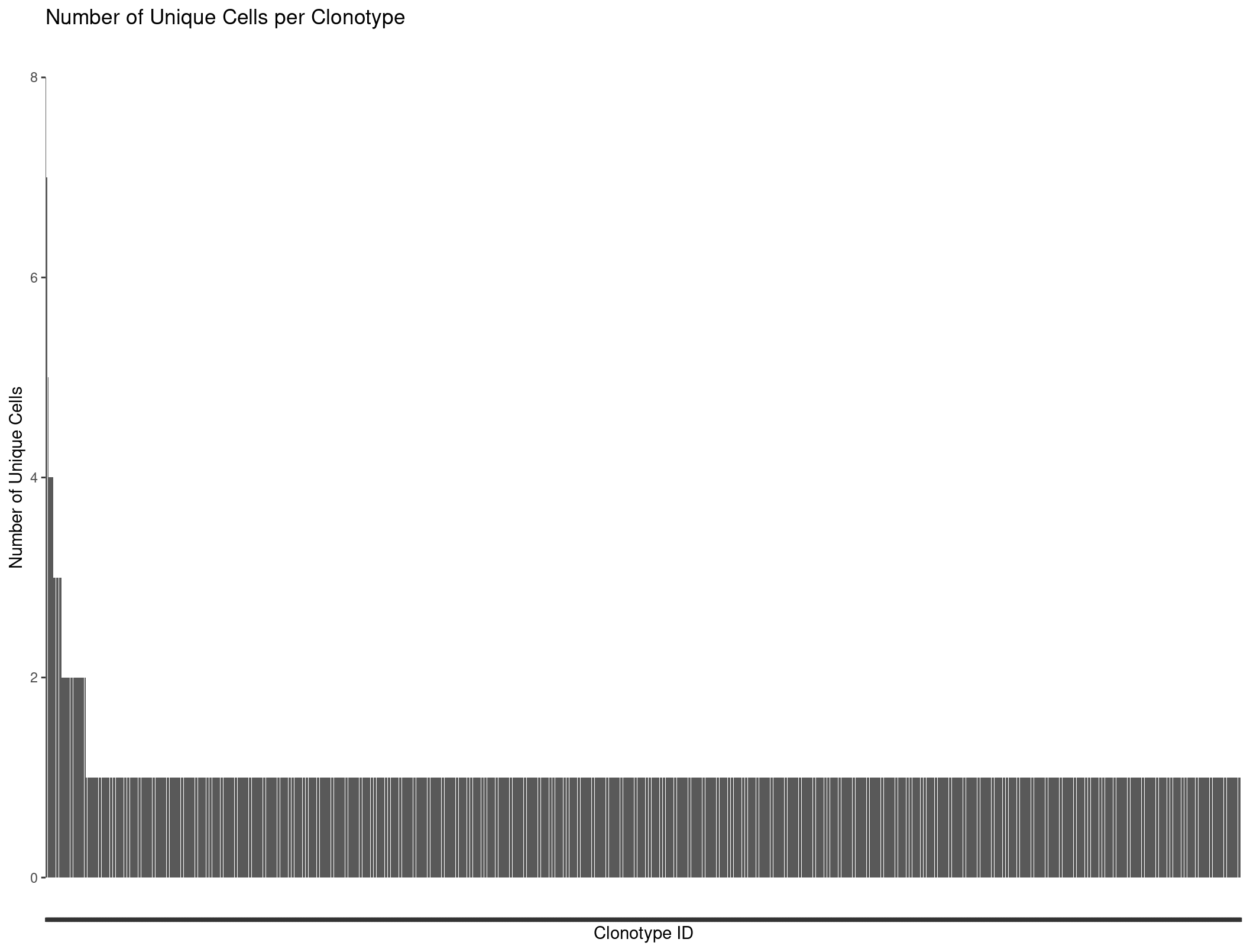
We can plot all our clonotypes to see the general distribution of TCRs per cells. We see a majority of cells only have one clonotype assoicated with them.
ggplot(Rep1_ICB_clonotype_counts, aes(x = reorder(raw_clonotype_id, -cell_count), y = cell_count)) +
  geom_bar(stat = "identity") +
  labs(x = "Clonotype ID",
       y = "Number of Unique Cells",
       title = "Number of Unique Cells per Clonotype") +
  theme(axis.text.x=element_blank())
Our barplot is nice but we might want to produce more complicated graphs to better visualize our repertoire. This is where scRepertoire comes into play.
scRepertoire for TCR analysis
scRepertoire is one of the first packages that allows the combining of single cell RNA and immune profiling. We will use it to perform more complex exploration of the TCR diversity within our data.
Loading in data
First lets load in our data for all our replicates.
Rep1_ICB_t <- read.csv("data/single_cell_rna/clonotypes_t_posit/Rep1_ICB-t-filtered_contig_annotations.csv")
Rep1_ICBdT_t <- read.csv("data/single_cell_rna/clonotypes_t_posit/Rep1_ICBdT-t-filtered_contig_annotations.csv")
Rep3_ICB_t <- read.csv("data/single_cell_rna/clonotypes_t_posit/Rep3_ICB-t-filtered_contig_annotations.csv")
Rep3_ICBdT_t <- read.csv("data/single_cell_rna/clonotypes_t_posit/Rep3_ICBdT-t-filtered_contig_annotations.csv")
Rep5_ICB_t <- read.csv("data/single_cell_rna/clonotypes_t_posit/Rep5_ICB-t-filtered_contig_annotations.csv")
Rep5_ICBdT_t <- read.csv("data/single_cell_rna/clonotypes_t_posit/Rep5_ICBdT-t-filtered_contig_annotations.csv")

# create a list of all samples' TCR data
TCR.contigs <- list(Rep1_ICB_t, Rep1_ICBdT_t, Rep3_ICB_t, Rep3_ICBdT_t, Rep5_ICB_t, Rep5_ICBdT_t)
Combining contigs into clones
Use scRepertoire’s combineTCR function to create an object with all samples’ TCR data. Note the additional filtering parameters: removeNA will remove any chain with NA values, removeMulti will remove barcodes with greater than 2 chains, and filterMulti will allow for the selection of the 2 corresponding chains with the highest expression for a single barcode.
We will set filterMulti to TRUE to avoid the confusing cases where there are multiple chains.
sample_names <- c("Rep1_ICB", "Rep1_ICBdT", "Rep3_ICB",
                 "Rep3_ICBdT", "Rep5_ICB", "Rep5_ICBdT")

combined.TCR <- combineTCR(TCR.contigs,
                           samples = sample_names,
                           removeNA = FALSE,
                           removeMulti = FALSE,
                           filterMulti = TRUE)

# view the object
View(combined.TCR[[1]])
So far we have not considered that we have filtered out some cells in our seurat object. Let’s filter our scRepertoire object to the same cells in our seurat object.
# Read in your Seurat object
# https://genomedata.org/cri-workshop/preprocessed_object.rds
rep135 <- readRDS("outdir_single_cell_rna/preprocessed_object.rds")

combined.TCR_filter <- combined.TCR # create a variable to hold our filtered object

index <- 1 # set an index for accessing our combined.TCR object
for (sample in sample_names) {

  print(paste0("Sample Name: ", sample))

  screp_barcodes <- combined.TCR[[index]]$barcode
  print(paste0("Number of barcodes in scRep obj: ", length(unique(screp_barcodes))))

  seurat_barcodes <- rownames(rep135@meta.data[rep135@meta.data$orig.ident == sample, ])
  print(paste0("Number of barcodes in seurat obj: ", length(seurat_barcodes)))

  TCR_clonotype_barcodes_filtered <- subset(combined.TCR[[index]], screp_barcodes %in% seurat_barcodes)

  print(paste0("Number of rows in scRep obj after filtering: ", nrow(TCR_clonotype_barcodes_filtered)))

  combined.TCR_filter[[index]] <- TCR_clonotype_barcodes_filtered

  index <- index + 1
}
[1] "Sample Name: Rep1_ICB"
[1] "Number of barcodes in scRep obj: 2586"
[1] "Number of barcodes in seurat obj: 2986"
[1] "Number of rows in scRep obj after filtering: 2397"
[1] "Sample Name: Rep1_ICBdT"
[1] "Number of barcodes in scRep obj: 959"
[1] "Number of barcodes in seurat obj: 3106"
[1] "Number of rows in scRep obj after filtering: 912"
[1] "Sample Name: Rep3_ICB"
[1] "Number of barcodes in scRep obj: 3607"
[1] "Number of barcodes in seurat obj: 5680"
[1] "Number of rows in scRep obj after filtering: 3506"
[1] "Sample Name: Rep3_ICBdT"
[1] "Number of barcodes in scRep obj: 3004"
[1] "Number of barcodes in seurat obj: 5072"
[1] "Number of rows in scRep obj after filtering: 2945"
[1] "Sample Name: Rep5_ICB"
[1] "Number of barcodes in scRep obj: 248"
[1] "Number of barcodes in seurat obj: 1794"
[1] "Number of rows in scRep obj after filtering: 241"
[1] "Sample Name: Rep5_ICBdT"
[1] "Number of barcodes in scRep obj: 2686"
[1] "Number of barcodes in seurat obj: 4547"
[1] "Number of rows in scRep obj after filtering: 2596"
We can compare the number of clonotypes scRepertoire calls compred to cellranger.
nrow(Rep1_ICB_clonotype_counts)
nrow(combined.TCR[[1]])
nrow(combined.TCR_filter[[1]])
> nrow(Rep1_ICB_clonotype_counts)
[1] 2444
> nrow(combined.TCR[[1]])
[1] 2586
> nrow(combined.TCR_filter[[1]])
[1] 2397
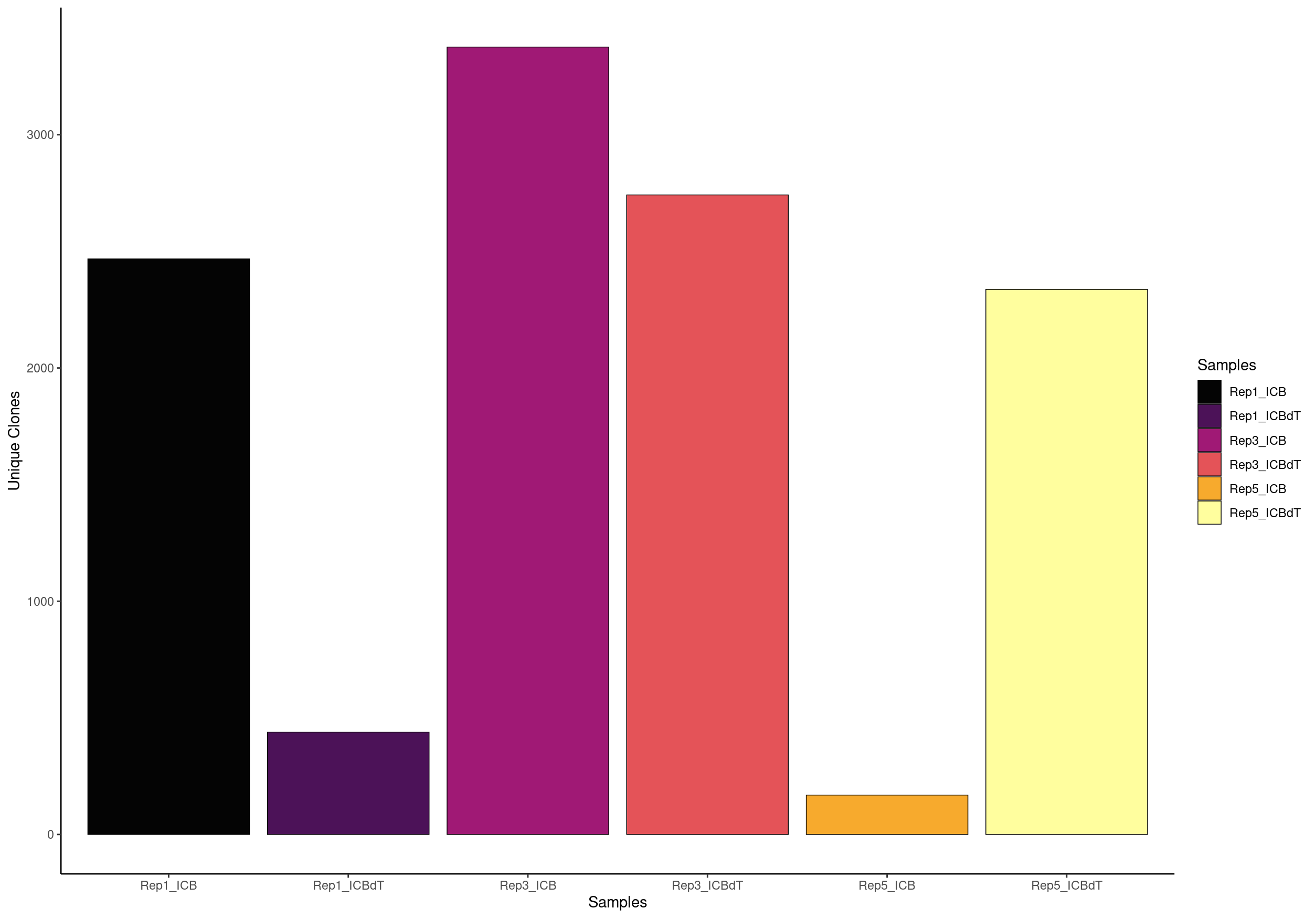
Visualize the Number of Clones
scRepertoire defines clones as TCRs with shared/trackable complementarity-determining region 3 (CDR3) sequences. You can define clones using the amino acid sequence (aa), nucleotide (nt), or the V(D)JC genes (genes). The latter genes would be a more permissive definition of “clones”, as multiple amino acid or nucleotide sequences can result from the same gene combination. You can also use a combination of the V(D)JC genes and nucleotide sequence (strict). scRepertoire also allows for the users to select both or individual chains to examine.
clonalQuant(combined.TCR_filter,
            cloneCall="aa",
            chain = "both",
            scale = FALSE)
For the TCR analysis, Freshour et al. 2023. excluded samples containing less than 1,500 TCR+ cells after filtering. We found that the majority of samples with less than 1,500 cells did not appear to have had their naive T cell populations captured during sequencing, which could lead to a skewed appearance of clonal expansion among the T cell populations that were captured
# OR view the relative percent of unique clones scaled by the total size of the clonal repertoire
clonalQuant(combined.TCR_filter,
            cloneCall="aa",
            chain = "both",
            scale = TRUE)

# OR export the counts as a table to view the absolute amount
clonalQuant(combined.TCR_filter,
            cloneCall="aa",
            chain = "both",
            scale = TRUE,
            exportTable = TRUE)
Here we see that contigs is our unique clonotypes and total is the number of cells that have a TCR assocaited with them.
  contigs     values total   scaled
1    2339   Rep1_ICB  2397 97.58031
2     429 Rep1_ICBdT   912 47.03947
3    3282   Rep3_ICB  3506 93.61095
4    2687 Rep3_ICBdT  2945 91.23939
5     164   Rep5_ICB   241 68.04979
6    2260 Rep5_ICBdT  2596 87.05701
Try changing the cloneCall argument to see how that changes the number of clones
Visualizing the proportion of the repertoire taken up by a specific clone
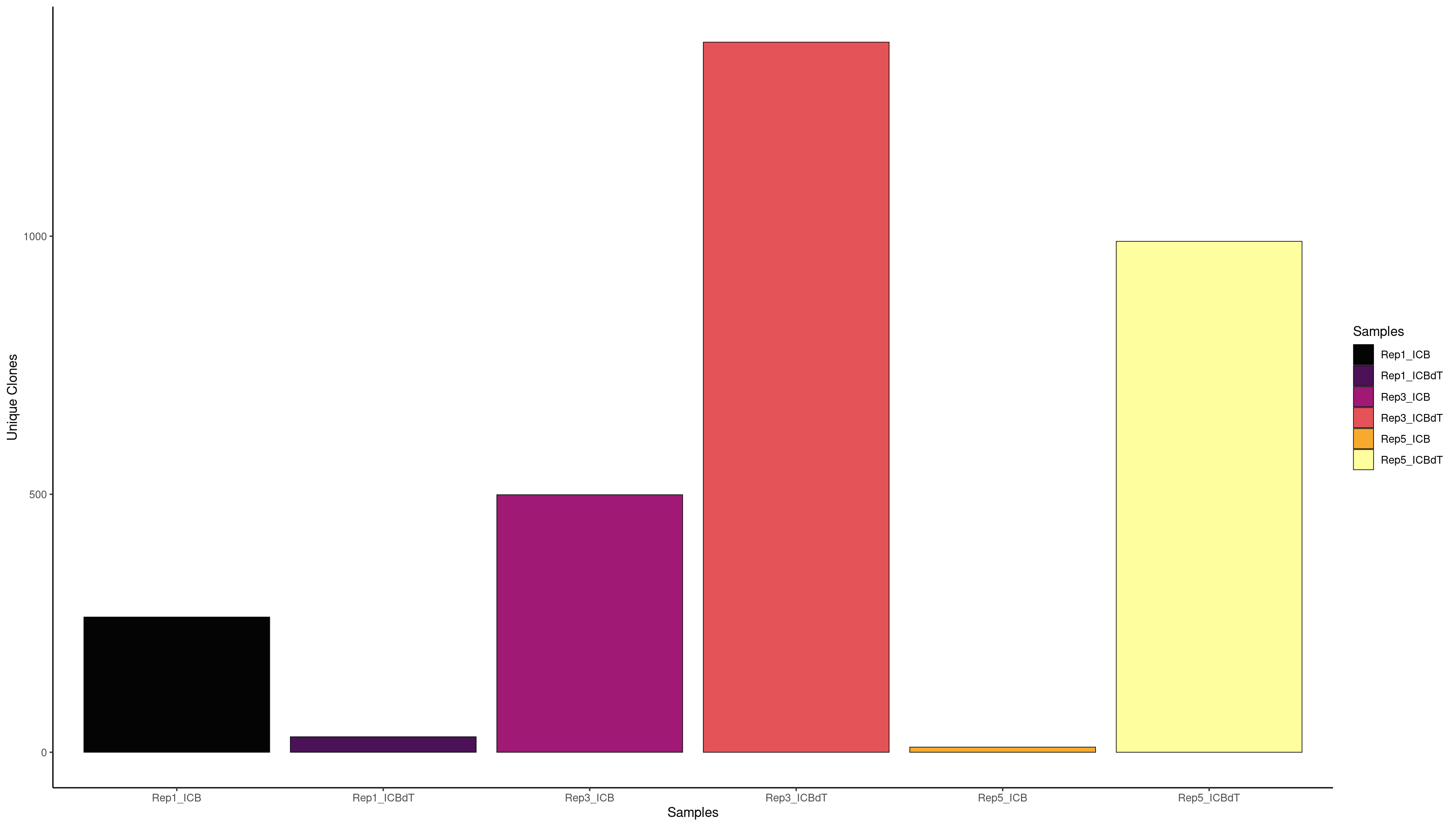
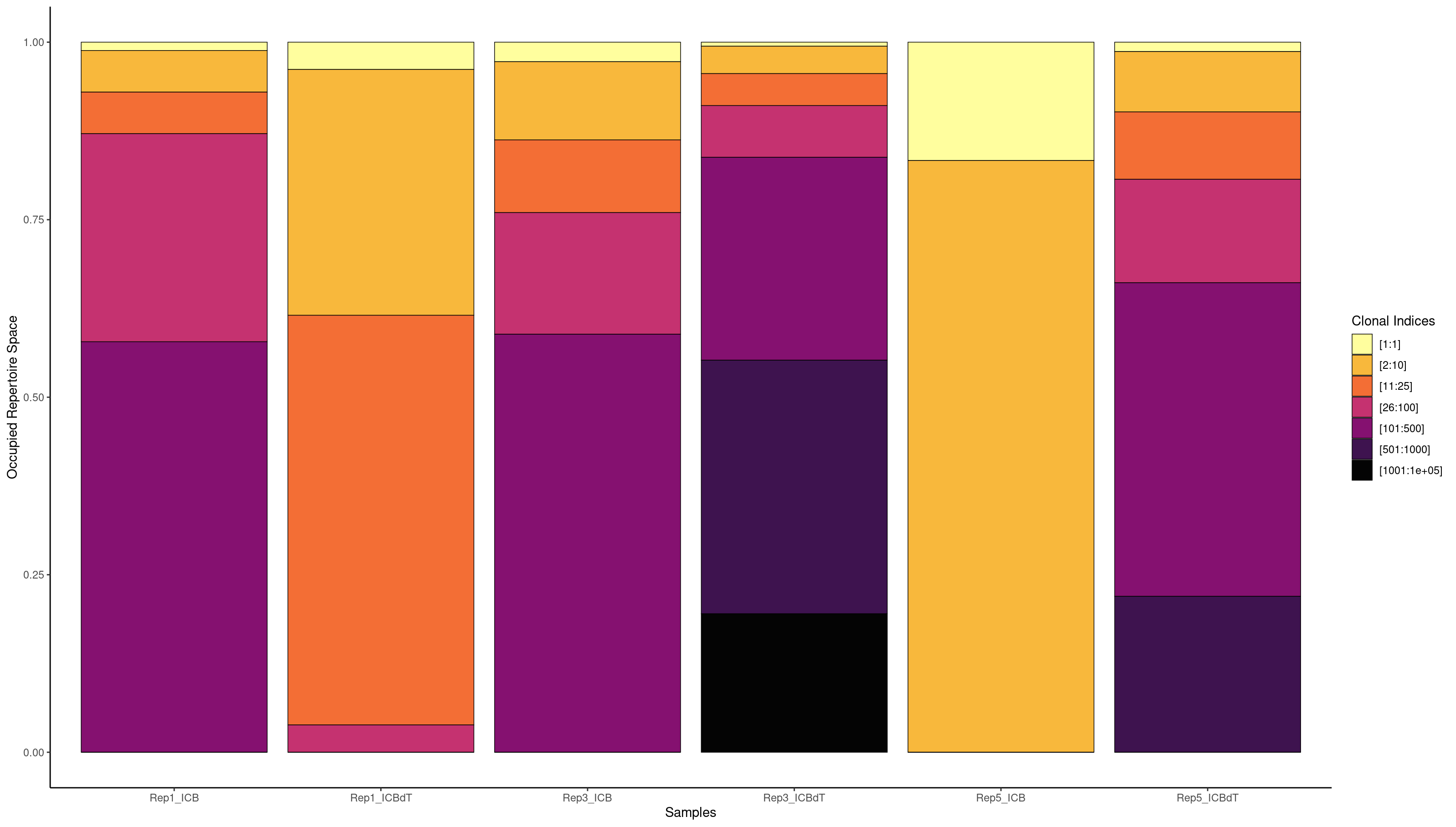
We are interested in understanding if there is a T cell response in our data. If there was a T cell response, we might see a single clonotype in a large portion of cells. Earlier we used a barplot to see how many cells each clonotype was seen in. Now we will use screpertoire’s clonalProportion function to produce stacked barplots visualizing how much space each clone is taking up.
We are going to split up our clones in the same way as Freshour et al. 2023, remembering that 1 here means clonotype1 which is assigned to our top clonotype.
clonalProportion(combined.TCR_filter, cloneCall = "aa", clonalSplit = c(1, 10, 25, 100, 500, 1000, 1e+05))
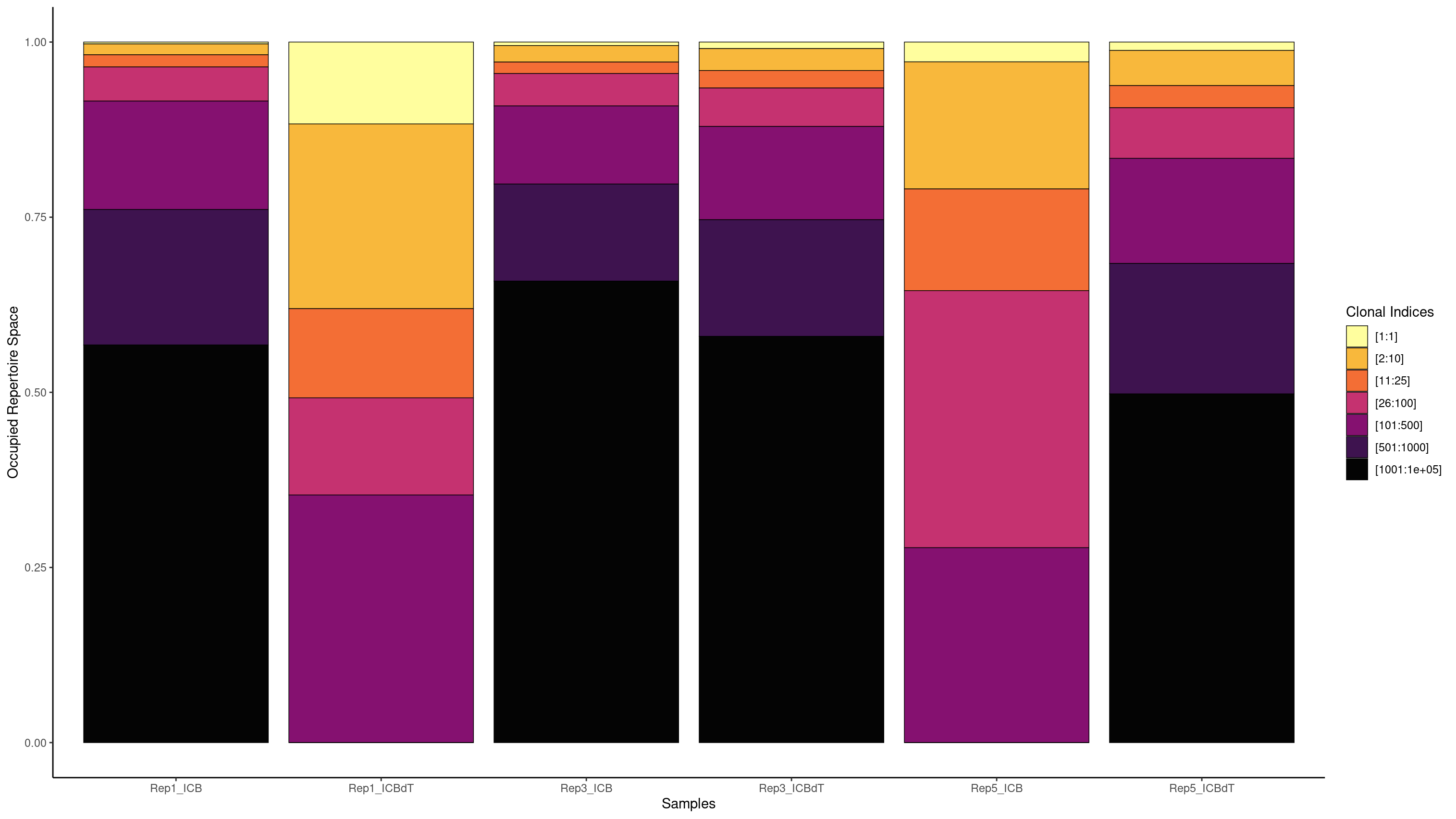
clonalProportion(combined.TCR_filter, cloneCall = "aa", clonalSplit = c(1, 10, 25, 100, 500, 1000, 1e+05), exportTable=TRUE)
           [1:1] [2:10] [11:25] [26:100] [101:500] [501:1000] [1001:1e+05]
Rep1_ICB       5     30      32       91       400        500         1339
Rep1_ICBdT   103    244     117      119       329          0            0
Rep3_ICB      18     85      59      162       400        500         2282
Rep3_ICBdT    28     93      75      162       400        500         1687
Rep5_ICB       7     43      36       91        64          0            0
Rep5_ICBdT    31    127      85      193       400        500         1260
We see the highest amount of expansion in Rep1_ICBdT and Rep5_ICB. However, from our counts barplots, we know that these samples have very few number of TCRs called, making this data untrustworthy. For the other samples, we see very little expansion of a single clonotype.
Understanding our BCR data
Now lets perform a similar analysis for our BCRs, keeping in mind the difference between BCRs and TCRs. BCRs can be hard to group because of somatic hypermutation which introduces multiple mutations during B cell maturation.
Rep1_ICB_b <- read.csv("data/single_cell_rna/clonotypes_b_posit/Rep1_ICB-b-filtered_contig_annotations.csv")
Rep1_ICBdT_b <- read.csv("data/single_cell_rna/clonotypes_b_posit/Rep1_ICBdT-b-filtered_contig_annotations.csv")
Rep3_ICB_b <- read.csv("data/single_cell_rna/clonotypes_b_posit/Rep3_ICB-b-filtered_contig_annotations.csv")
Rep3_ICBdT_b <- read.csv("data/single_cell_rna/clonotypes_b_posit/Rep3_ICBdT-b-filtered_contig_annotations.csv")
Rep5_ICB_b <- read.csv("data/single_cell_rna/clonotypes_b_posit/Rep5_ICB-b-filtered_contig_annotations.csv")
Rep5_ICBdT_b <- read.csv("data/single_cell_rna/clonotypes_b_posit/Rep5_ICBdT-b-filtered_contig_annotations.csv")

colnames(Rep1_ICB_t) # TCR column names
colnames(Rep1_ICB_b) # BCR column names
View(Rep1_ICB_b)
Notice that our column names are the exact same for TCRs and BCRs but when you view the BCR data we see that of course the gene names have changed and the chains are either IGH (heavy chain) or IGK/IGL (light chain).
All cells should either have a IGH/IGK combination or IGH/IGL combination.
Let’s use our R skills to again count the unique cells per clonotype.
Rep1_ICB_clonotype_counts <- Rep1_ICB_b %>%
  distinct(barcode, raw_clonotype_id) %>%  # First get unique barcode-clonotype pairs
  group_by(raw_clonotype_id) %>%
  summarize(cell_count = n()) %>%
  arrange(desc(cell_count))  # Sort by count for better visualization

head(Rep1_ICB_clonotype_counts)
# A tibble: 6 × 2
  raw_clonotype_id cell_count
  <chr>                 <int>
1 clonotype1              137
2 clonotype2                4
3 clonotype3                3
4 clonotype10               2
5 clonotype11               2
6 clonotype12               2
ggplot(Rep1_ICB_clonotype_counts, aes(x = reorder(raw_clonotype_id, -cell_count), y = cell_count)) +
  geom_bar(stat = "identity") +
  labs(x = "Clonotype ID",
       y = "Number of Unique Cells",
       title = "Number of Unique Cells per Clonotype") +
  theme(axis.text.x=element_blank())
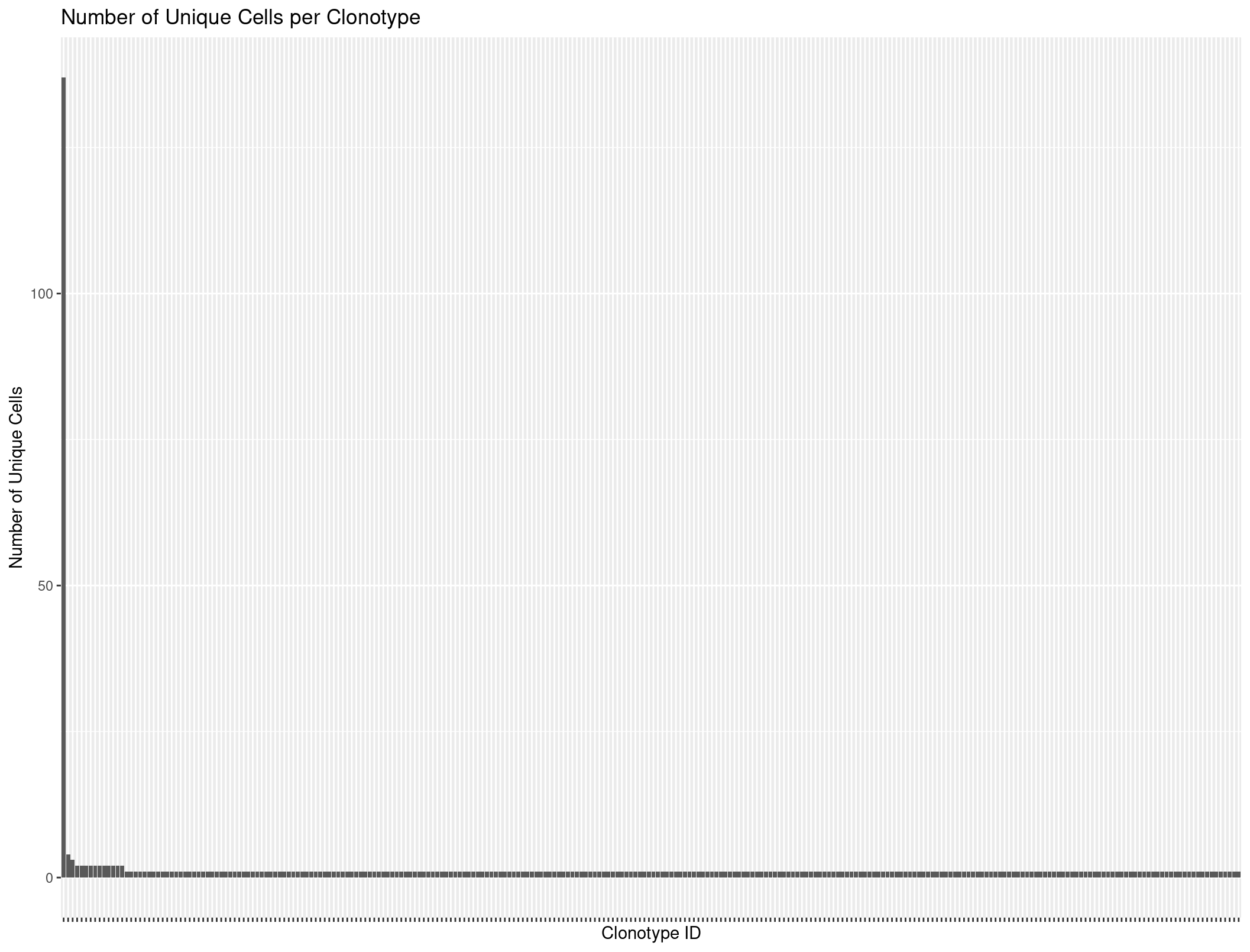
When we plot it looks like there might be some evidence of expansion. However, lets use scRepertoire to look more in depth.
scRepertoire for BCR analysis
Unlike combineTCR, combineBCR produces a column called CTstrict of an index of nucleotide sequence and the corresponding V gene. This index automatically calculates the Levenshtein distance between sequences with the same V gene and will index sequences using a normalized Levenshtein distance with the same ID. After which, clone clusters are called using the components function. Clones that are clustered across multiple sequences will then be labeled with “Cluster” in the CTstrict header. We use the threshold parameter to set the normalized edit distance to consider, where the higher the number the more similarity of sequence will be used for clustering.
BCR.contigs <- list(Rep1_ICB_b, Rep1_ICBdT_b, Rep3_ICB_b, Rep3_ICBdT_b, Rep5_ICB_b, Rep5_ICBdT_b)

sample_names <- c("Rep1_ICB", "Rep1_ICBdT", "Rep3_ICB", "Rep3_ICBdT", "Rep5_ICB", "Rep5_ICBdT")

combined.BCR_85 <- combineBCR(BCR.contigs,
                              samples = sample_names,
                              threshold = 0.85) # more unique clonotypes

combined.BCR_05 <- combineBCR(BCR.contigs,
                              samples = sample_names,
                              threshold = 0.05) # less unique clonotypes

clonalQuant(combined.BCR_85,
            cloneCall="strict",
            chain = "both",
            scale = FALSE,
            exportTable = TRUE)

clonalQuant(combined.BCR_05,
              cloneCall="strict",
              chain = "both",
              scale = FALSE,
              exportTable = TRUE)
  contigs     values total
1     262   Rep1_ICB   414
2      30 Rep1_ICBdT    30
3     499   Rep3_ICB   687
4    1376 Rep3_ICBdT  1537
5      10   Rep5_ICB    11
6     990 Rep5_ICBdT  1374

  contigs     values total
1     248   Rep1_ICB   414
2      30 Rep1_ICBdT    30
3     462   Rep3_ICB   687
4    1064 Rep3_ICBdT  1537
5       9   Rep5_ICB    11
6     830 Rep5_ICBdT  1374
When we lower the threshold there are less unique clonotypes. What the best threshold is depends on what data you are looking at. We will use the default of 0.85.
We will also filter the scRepertoire BCR object to the same barcodes as those in the single cell object.
combined.BCR_filter <- combined.BCR_85 # create a variable to hold our filtered object

index <- 1 # set an index for accessing our combined.BCR object
for (sample in sample_names) {

  print(paste0("Sample Name: ", sample))

  screp_barcodes <- combined.BCR_85[[index]]$barcode
  print(paste0("Number of barcodes in scRep obj: ", length(unique(screp_barcodes))))

  seurat_barcodes <- rownames(rep135@meta.data[rep135@meta.data$orig.ident == sample, ])
  print(paste0("Number of barcodes in seurat obj: ", length(seurat_barcodes)))

  BCR_clonotype_barcodes_filtered <- subset(combined.BCR_85[[index]], screp_barcodes %in% seurat_barcodes)

  print(paste0("Number of rows in scRep obj after filtering: ", nrow(BCR_clonotype_barcodes_filtered)))

  combined.BCR_filter[[index]] <- BCR_clonotype_barcodes_filtered

  index <- index + 1
}
[1] "Sample Name: Rep1_ICB"
[1] "Number of barcodes in scRep obj: 414"
[1] "Number of barcodes in seurat obj: 2986"
[1] "Number of rows in scRep obj after filtering: 256"
[1] "Sample Name: Rep1_ICBdT"
[1] "Number of barcodes in scRep obj: 30"
[1] "Number of barcodes in seurat obj: 3106"
[1] "Number of rows in scRep obj after filtering: 26"
[1] "Sample Name: Rep3_ICB"
[1] "Number of barcodes in scRep obj: 687"
[1] "Number of barcodes in seurat obj: 5680"
[1] "Number of rows in scRep obj after filtering: 654"
[1] "Sample Name: Rep3_ICBdT"
[1] "Number of barcodes in scRep obj: 1537"
[1] "Number of barcodes in seurat obj: 5072"
[1] "Number of rows in scRep obj after filtering: 1400"
[1] "Sample Name: Rep5_ICB"
[1] "Number of barcodes in scRep obj: 11"
[1] "Number of barcodes in seurat obj: 1794"
[1] "Number of rows in scRep obj after filtering: 6"
[1] "Sample Name: Rep5_ICBdT"
[1] "Number of barcodes in scRep obj: 1374"
[1] "Number of barcodes in seurat obj: 4547"
[1] "Number of rows in scRep obj after filtering: 906"
There are way fewer BCRs called compared to TCRs.
Visualize the Number of Clones
clonalQuant(combined.BCR_filter,
            cloneCall="strict",
            chain = "both",
            scale = FALSE)
clonalQuant(combined.BCR_filter,
            cloneCall="aa",
            chain = "both",
            scale = TRUE,
            exportTable = TRUE)

# Note that our threshold will only change the number called in our strict category
clonalQuant(combined.BCR_filter,
            cloneCall="strict",
            chain = "both",
            scale = TRUE,
            exportTable = TRUE)
  contigs     values total    scaled
1     253   Rep1_ICB   256  98.82812
2      26 Rep1_ICBdT    26 100.00000
3     564   Rep3_ICB   654  86.23853
4    1333 Rep3_ICBdT  1400  95.21429
5       6   Rep5_ICB     6 100.00000
6     793 Rep5_ICBdT   906  87.52759

  contigs     values total    scaled
1     248   Rep1_ICB   256  96.87500
2      26 Rep1_ICBdT    26 100.00000
3     485   Rep3_ICB   654  74.15902
4    1273 Rep3_ICBdT  1400  90.92857
5       6   Rep5_ICB     6 100.00000
6     699 Rep5_ICBdT   906  77.15232
We can also look at what clones are expanded but we have such a small number of BCRs that most of this data is probably untrustworthy.
clonalProportion(combined.BCR_filter, cloneCall = "strict", clonalSplit = c(1, 10, 25, 100, 500, 1000, 1e+05))
Adding the BCR and TCR Data to your Seurat object
We will now add the BCR and TCR information which has been handled by scRepertoire so far to our Seurat object.
Use the combineExpression function to add the TCR data to your Seurat object. The columns CTgene, CTnt, CTaa, CTstrict, clonalProportion, clonalFrequency, and cloneSize data will be added to your Seurat object’s metadata. Notice you can also decide the bins for grouping based on proportion or frequency of the TCRs (or BCRs).
Here we group by frequency:
rep135 <- combineExpression(combined.TCR, rep135,
                         cloneCall="aa", proportion = FALSE,
                         group.by = "sample",
                         cloneSize=c(Single=1, Small=5, Medium=20, Large=100, Hyperexpanded=500))

colnames(rep135@meta.data)
Since we want to add both BCR and TCR information we have to rename the columns to make it clear since scRepertoire uses the same column names for BCR and TCR data.
columns_to_modify <- c("CTgene", "CTnt", "CTaa", "CTstrict", "clonalProportion", "clonalFrequency", "cloneSize")
names(rep135@meta.data)[names(rep135@meta.data) %in% columns_to_modify] <- paste0(columns_to_modify, "_TCR")

colnames(rep135@meta.data) # make sure the column names are changed
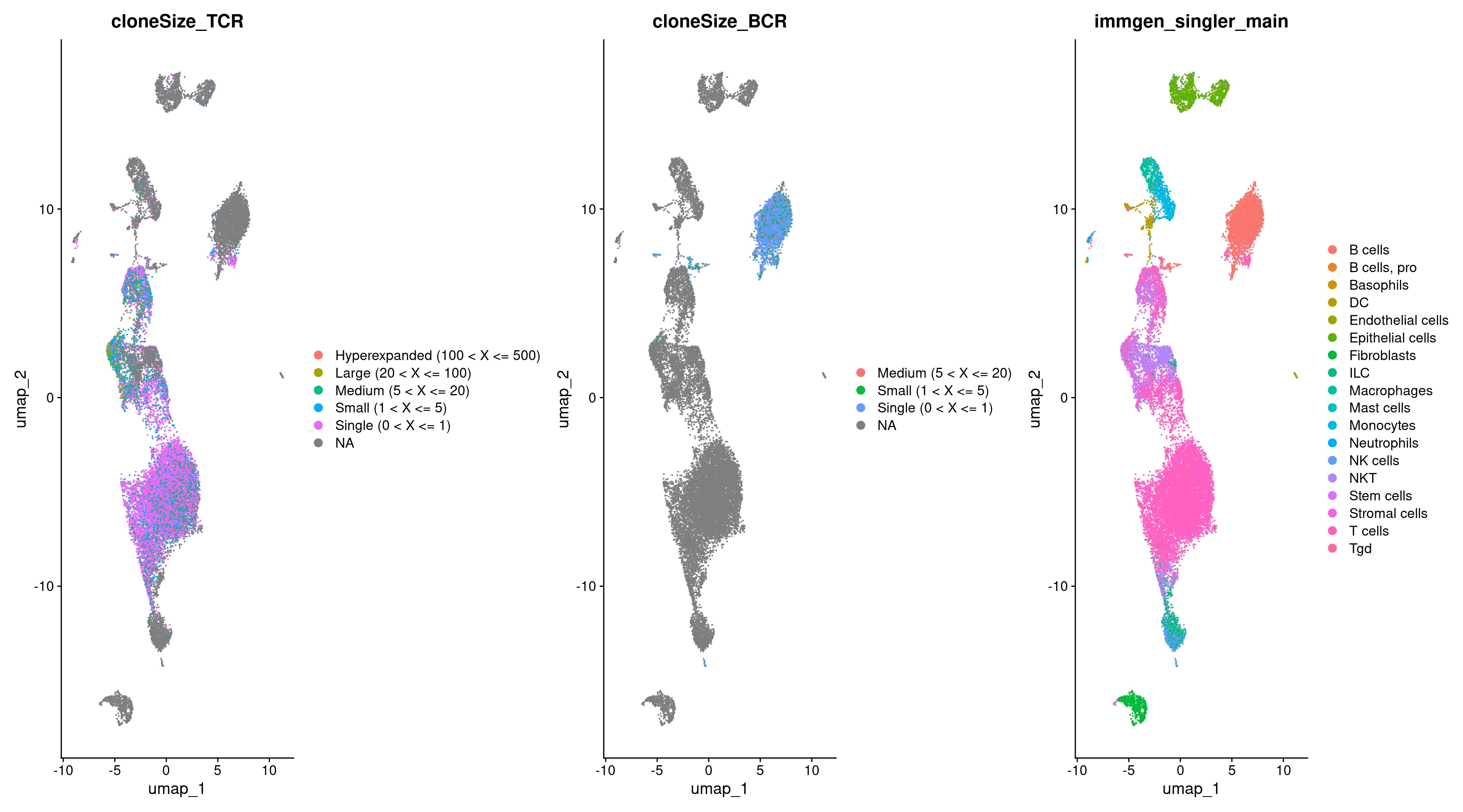
We can now plot the cells with TCRs and compare that to our cell type annotations. Indeed, we see a majority of TCRs in the same clusters which are called T cells!
DimPlot(rep135, group.by = c("cloneSize_TCR", "immgen_singler_main"))
Let’s repeat the same steps with the BCR data.
rep135 <- combineExpression(combined.BCR_85, rep135,
                              cloneCall="aa", proportion = FALSE,
                              group.by = "sample",
                              cloneSize=c(Single=1, Small=5, Medium=20, Large=100, Hyperexpanded=500))

names(rep135@meta.data)[names(rep135@meta.data) %in% columns_to_modify] <- paste0(columns_to_modify, "_BCR")
colnames(rep135@meta.data) # make sure the column names are changed
Now let’s visualize the TCR, BCR, and cell type annotations with a UMAP.
DimPlot(rep135, group.by = c("cloneSize_TCR", "cloneSize_BCR", "immgen_singler_main"))
Exercise: Create a custom bar graph with BCR and TCR information
So now we have this data, but how do we use it? How could we use the information our Seurat object already holds to analysis our BCR/TCR information further?
Say we want to create a bar plot that shows the number of clones by each cell type. So we want the x-axis to be the number of clones and the y-axis to be counts of BCR or TCRs.
Let’s start by deciding what information we need to make this graph.
colnames(rep135@meta.data)
Create a dataframe that contains just that information, mainly for ease. Here we are going to grab the cell type labels and the amino acid sequences for the CDR3s.
rep135_TCR_clones <- rep135@meta.data[, c("CTaa_TCR", "immgen_singler_main")]

head(rep135_TCR_clones)
The dataframe should look something like this, where we have some cells with a TCR and their cell type label.
                                                   CTaa_TCR immgen_singler_main
Rep1_ICBdT_AAACCTGAGCCAACAG-1  CALGAVSAGNKLTF_CASRGGAYAEQFF                 NKT
Rep1_ICBdT_AAACCTGAGCCTTGAT-1                          <NA>             B cells
Rep1_ICBdT_AAACCTGAGTACCGGA-1                          <NA>         Fibroblasts
Rep1_ICBdT_AAACCTGCACGGCCAT-1                          <NA>            NK cells
Rep1_ICBdT_AAACCTGCACGGTAAG-1 CATDGGTGSNRLTF_CASSYGQGDSDYTF             T cells
Rep1_ICBdT_AAACCTGCATGCCACG-1                          <NA>         Fibroblasts
First, we should use groupby to group our data into the categories that we want to plot.
rep135_TCR_clones %>%
  group_by(immgen_singler_main)
# A tibble: 23,185 × 2
# Groups:   immgen_singler_main [18]
   CTaa_TCR                       immgen_singler_main
   <chr>                          <chr>
 1 CALGAVSAGNKLTF_CASRGGAYAEQFF   NKT
 2 NA                             B cells
 3 NA                             Fibroblasts
 4 NA                             NK cells
 5 CATDGGTGSNRLTF_CASSYGQGDSDYTF  T cells
 6 NA                             Fibroblasts
 7 CAARLGMSNYNVLYF_CASSQTGGDERLFF T cells
 8 NA                             Neutrophils
 9 NA                             Fibroblasts
10 CALGAVSAGNKLTF_CASRGGAYAEQFF   NKT
# ℹ 23,175 more rows
# ℹ Use `print(n = ...)` to see more rows
Then we want to use the summarise function to create a count of how many TCRs we see:
rep135_TCR_clones %>%
    group_by(immgen_singler_main) %>%
    summarise(Count = n())
# A tibble: 18 × 2
   immgen_singler_main Count
   <chr>               <int>
 1 B cells              3253
 2 B cells, pro            3
 3 Basophils              37
 4 DC                    295
 5 Endothelial cells      71
 6 Epithelial cells     1238
 7 Fibroblasts           589
 8 ILC                   763
 9 Macrophages           459
10 Mast cells             11
11 Monocytes             633
12 NK cells              565
13 NKT                  2249
14 Neutrophils            92
15 Stem cells              2
16 Stromal cells          18
17 T cells             12714
18 Tgd                   193
This looks good! Let’s plot it with a barplot:
TCR_celltypes_summary <- rep135_TCR_clones %>%
group_by(immgen_singler_main) %>%
summarise(Count = n())
ggplot(TCR_celltypes_summary, aes(x = immgen_singler_main, y = Count)) +
geom_bar(stat = "identity", fill = "skyblue") +
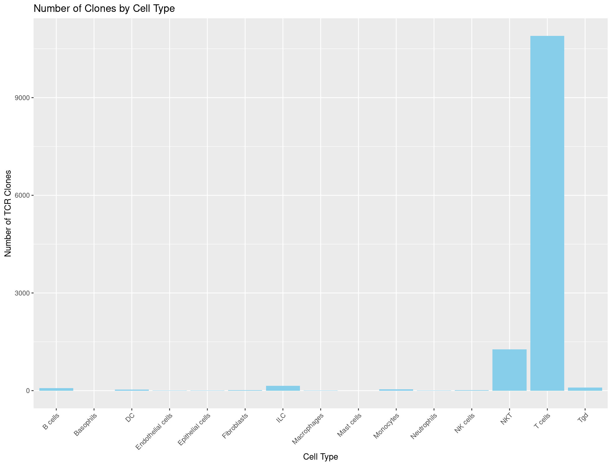
labs(x = "Cell Type", y = "Number of TCR Clones", title = "Number of Clones by Cell Type") +
theme(axis.text.x = element_text(angle = 45, hjust = 1)) # adjust the x-axis labels so that they are not overlapping each other
Hmmmmmmmmm, this looks a little suspicious. There are a lot of B cells with TCRs… maybe our summarise function was incorrect?
Let’s check the counts when we sum just our cell types column.
table(rep135@meta.data$immgen_singler_main)
Unfortunately, those are the same numbers as our summary dataframe above. We want to be counting how many TCRs are seen per cell type not how many of each cell type we have. What do you think could be the problem?
          B cells      B cells, pro         Basophils                DC Endothelial cells  Epithelial cells       Fibroblasts               ILC       Macrophages
             3253                 3                37               295                71              1238               589               763               459
       Mast cells         Monocytes       Neutrophils          NK cells               NKT        Stem cells     Stromal cells           T cells               Tgd
               11               633                92               565              2249                 2                18             12714               193
# A tibble: 23,185 × 2
# Groups:   immgen_singler_main [18]
   CTaa_TCR                       immgen_singler_main
   <chr>                          <chr>
 1 CALGAVSAGNKLTF_CASRGGAYAEQFF   NKT
 2 NA                             B cells
 3 NA                             Fibroblasts
 4 NA                             NK cells
 5 CATDGGTGSNRLTF_CASSYGQGDSDYTF  T cells
 6 NA                             Fibroblasts
 7 CAARLGMSNYNVLYF_CASSQTGGDERLFF T cells
 8 NA                             Neutrophils
 9 NA                             Fibroblasts
10 CALGAVSAGNKLTF_CASRGGAYAEQFF   NKT
# ℹ 23,175 more rows
# ℹ Use `print(n = ...)` to see more rows
It seems that those pesky NAs are being counted during our summarise command which we don’t want. If a cell has no TCR it should not be counted. Throwing in a na.omit() should do the trick!
rep135_TCR_clones %>%
    group_by(immgen_singler_main) %>% na.omit()
# A tibble: 12,597 × 2
# Groups:   immgen_singler_main [15]
   CTaa_TCR                                  immgen_singler_main
   <chr>                                     <chr>
 1 CALGAVSAGNKLTF_CASRGGAYAEQFF              NKT
 2 CATDGGTGSNRLTF_CASSYGQGDSDYTF             T cells
 3 CAARLGMSNYNVLYF_CASSQTGGDERLFF            T cells
 4 CALGAVSAGNKLTF_CASRGGAYAEQFF              NKT
 5 CAARLGMSNYNVLYF_CASSQTGGDERLFF            DC
 6 CAMREGSNNRIFF;CALSGANNNNAPRF_CASSYRGFDYTF T cells
 7 CAAHSNYQLIW_CASSPGTGGYEQYF                NKT
 8 CAVKNNRIFF_CASGDARGVEQYF                  ILC
 9 CAASEGGNYKPTF_CASSRDRYAEQFF               NKT
10 CARTNTGYQNFYF_CASSPHNSPLYF                Monocytes
# ℹ 12,587 more rows
# ℹ Use `print(n = ...)` to see more rows
That looks much better. So all together we have a command that looks like this to get the data into the correct format for the barplot.
# Count occurrences of each cell type
cell_type_counts_TCR <- rep135_TCR_clones %>%
  group_by(immgen_singler_main) %>% na.omit() %>%
  summarise(Count = n())
Finally, we get to plot something!
ggplot(cell_type_counts_TCR, aes(x = immgen_singler_main, y = Count)) +
  geom_bar(stat = "identity", fill = "skyblue") +
  labs(x = "Cell Type", y = "Number of TCR Clones", title = "Number of Clones by Cell Type") +
  theme(axis.text.x = element_text(angle = 45, hjust = 1))
And it looks great!
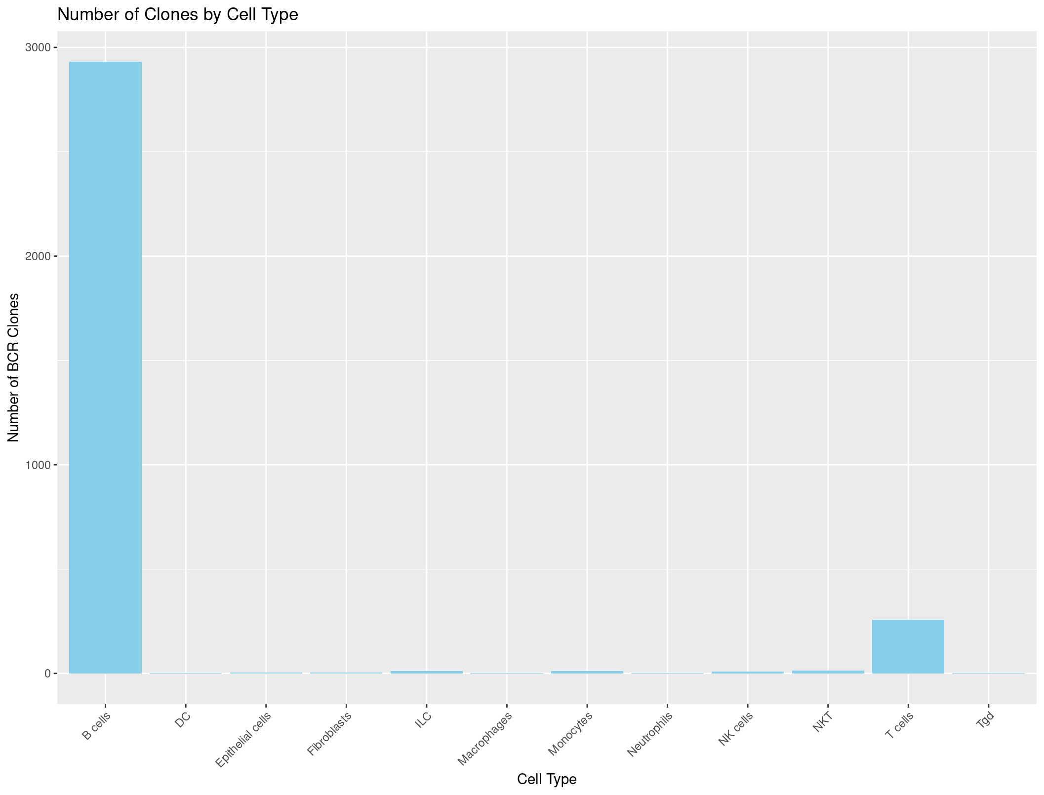
Now we can do the same thing with the BCR data.
rep135_BCR_clones <- rep135@meta.data[, c("CTaa_BCR", "immgen_singler_main")]

# Count occurrences of each cell type
cell_type_counts_BCR <- rep135_BCR_clones %>%
  group_by(immgen_singler_main) %>% na.omit() %>%
  summarise(Count = n())

# Plot
ggplot(cell_type_counts_BCR, aes(x = immgen_singler_main, y = Count)) +
  geom_bar(stat = "identity", fill = "skyblue") +
  labs(x = "Cell Type", y = "Number of BCR Clones", title = "Number of Clones by Cell Type") +
  theme(axis.text.x = element_text(angle = 45, hjust = 1))
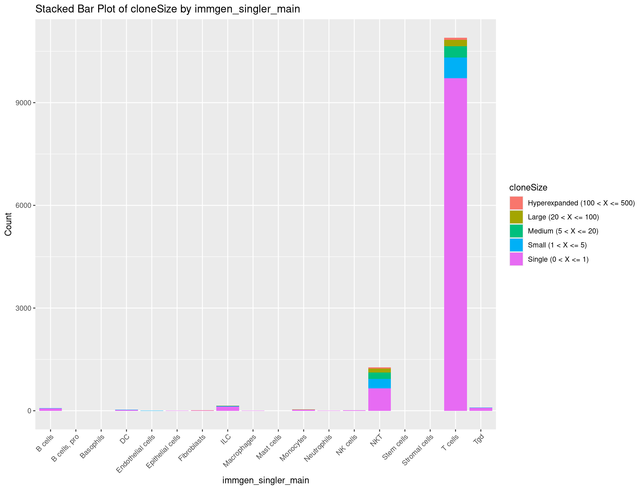
Bonus Exercise: Stacked bar plot of cell types by counts grouped by TCR clones
What if we wanted to see not just how many clones there are, but also the number of unique clones, and how many cells we see each unique clone in? Let’s create a stacked barplot that shows the number of clones for each cell type, but grouped by unique clones.
We can start by using the table function again.
rep135_TCR_clones <- rep135@meta.data[, c("CTaa_BCR", "immgen_singler_main", "cloneSize_TCR")]

table(rep135_TCR_clones$cloneSize_TCR)
Hyperexpanded (100 < X <= 500)          Large (20 < X <= 100)           Medium (5 < X <= 20)             Small (1 < X <= 5)
                           103                            315                            531                            917
           Single (0 < X <= 1)               None ( < X <= 0)
                         10731                              0
We see that most clones are only seen once, but if we look carefully there are some clones which are seen in mutiple cells. So we are on the right track. But we want these counts grouped by cell type. Can we run table with two parameters? (You might think this is silly but I genuinely couldn’t remember when I tried this the first time)
# Count occurrences of each cloneSize_TCR
cloneSize_immgen_table <- table(rep135_TCR_clones$cloneSize_TCR, rep135_TCR_clones$immgen_singler_main)

head(cloneSize_immgen_table)
                                 B cells B cells, pro Basophils   DC Endothelial cells Epithelial cells Fibroblasts  ILC Macrophages
  Hyperexpanded (100 < X <= 500)       0            0         1    2                 0                0           4    0           0
  Large (20 < X <= 100)                0            0         0    1                 0                0           1    4           0
  Medium (5 < X <= 20)                 3            0         0    3                 0                0           4    6           1
  Small (1 < X <= 5)                   9            0         0    2                 1                0           1   10           2
  Single (0 < X <= 1)                 68            0         0   27                 1                3           3  125           6
  None ( < X <= 0)                     0            0         0    0                 0                0           0    0           0

                                 Mast cells Monocytes Neutrophils NK cells  NKT Stem cells Stromal cells T cells  Tgd
  Hyperexpanded (100 < X <= 500)          0         1           0        1   37          0             0      57    0
  Large (20 < X <= 100)                   0         1           0        0  116          0             0     191    1
  Medium (5 < X <= 20)                    0         4           0        0  181          0             0     328    1
  Small (1 < X <= 5)                      0         2           0        1  281          0             0     604    4
  Single (0 < X <= 1)                     1        30           3       11  653          0             0    9712   88
  None ( < X <= 0)                        0         0           0        0    0          0             0       0    0
Well no way, that is exactly the summary we want. We still have a problem where we have a little too much information to be graphed in a way that is useful. How about we get rid of any row where there are 0 clones seen.
cloneSize_immgen_table <- cloneSize_immgen_table[-c(6), ]

head(cloneSize_immgen_table)
                                 B cells B cells, pro Basophils   DC Endothelial cells Epithelial cells Fibroblasts  ILC Macrophages
  Hyperexpanded (100 < X <= 500)       0            0         1    2                 0                0           4    0           0
  Large (20 < X <= 100)                0            0         0    1                 0                0           1    4           0
  Medium (5 < X <= 20)                 3            0         0    3                 0                0           4    6           1
  Small (1 < X <= 5)                   9            0         0    2                 1                0           1   10           2
  Single (0 < X <= 1)                 68            0         0   27                 1                3           3  125           6

                                 Mast cells Monocytes Neutrophils NK cells  NKT Stem cells Stromal cells T cells  Tgd
  Hyperexpanded (100 < X <= 500)          0         1           0        1   37          0             0      57    0
  Large (20 < X <= 100)                   0         1           0        0  116          0             0     191    1
  Medium (5 < X <= 20)                    0         4           0        0  181          0             0     328    1
  Small (1 < X <= 5)                      0         2           0        1  281          0             0     604    4
  Single (0 < X <= 1)                     1        30           3       11  653          0             0    9712   88
This is a little bit more manageable. Let’s make this a dataframe and clean it up to get ready to plot.
# Convert the filtered contingency table to a dataframe
cloneSize_immgen_df <- as.data.frame(cloneSize_immgen_table)

# Rename columns
colnames(cloneSize_immgen_df) <- c("cloneSize", "immgen_singler_main", "Count")
# Plot stacked bar plot
ggplot(cloneSize_immgen_df, aes(x = immgen_singler_main, y = Count, fill = cloneSize)) +
  geom_bar(stat = "identity") +
  labs(x = "immgen_singler_main", y = "Count", title = "Stacked Bar Plot of cloneSize by immgen_singler_main") +
  theme(axis.text.x = element_text(angle = 45, hjust = 1))
Data wrangling and visualization take a lot of finagling to get just right, especially as your dataset grows and your information becomes more complex. It usually takes some time to figure out how to visualize your data and then playing with that visualization to get it just right.
Resources
There are many, many more tools that can be used for TCR/BCR analysis. This github page summerizes a few!